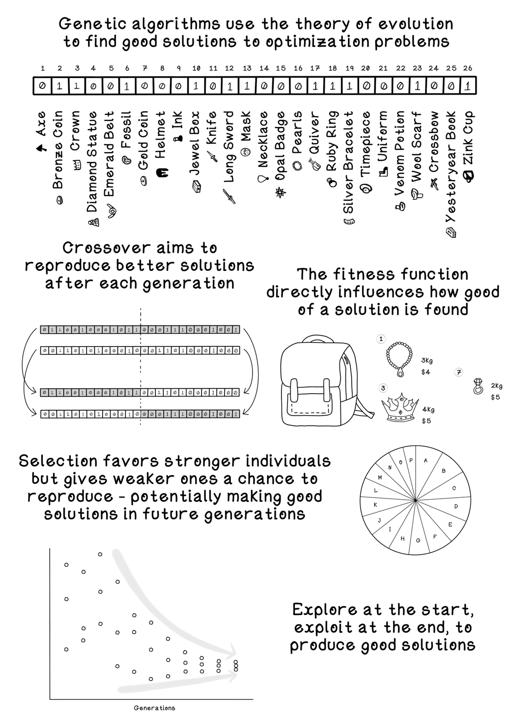
This chapter introduces evolutionary algorithms as computational analogs of natural selection, emphasizing that real evolution is a branching, variation-driven process where fitter variants tend to survive and reproduce. Translating this to computing, evolutionary algorithms search vast solution spaces by generating diverse candidates, scoring their fitness, selecting promising ones, and iterating over generations. They are stochastic, well-suited to complex optimization problems riddled with local optima, and aim for highly desirable—though not always provably optimal—solutions. The knapsack problem serves as a running example to illustrate how these methods navigate combinatorial explosions more efficiently than brute force.
At the core is careful encoding of solutions as chromosomes composed of genes (e.g., binary strings indicating item inclusion for knapsack), plus an initial population that respects constraints or is repaired/penalized if invalid. A fitness function measures solution quality (such as maximizing total value under a weight limit), after which probabilistic selection (notably roulette-wheel selection) favors fitter individuals while preserving diversity. Reproduction combines parents via crossover (single-point, two-point, or uniform) and introduces controlled randomness through mutation (bit flips or full flip-bit variants) to avoid premature convergence. Population models (steady-state vs. generational) and the diversity-to-convergence trajectory are managed to balance exploration and exploitation.
The full lifecycle repeatedly evaluates fitness, selects parents, reproduces and mutates offspring, then selects survivors for the next generation until a stopping condition is met (fixed generations, reaching a target fitness, or detecting stagnation). Compared with exhaustive enumeration, a well-configured genetic algorithm can reach strong solutions faster, accepting that “good enough” may be contextually sufficient. Performance hinges on thoughtful parameter choices: encoding scheme, population size and initialization, number of offspring, selection and survivor strategies, crossover and mutation methods and rates, and stopping criteria. Beyond knapsack-style packing, applications span logistics and routing, feature selection in machine learning, financial behavior modeling, and cipher cracking, with potential to integrate with other techniques such as neural networks.
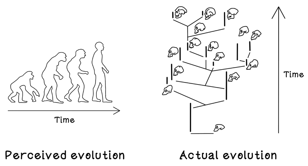
The idea of linear human evolution vs. actual human evolution
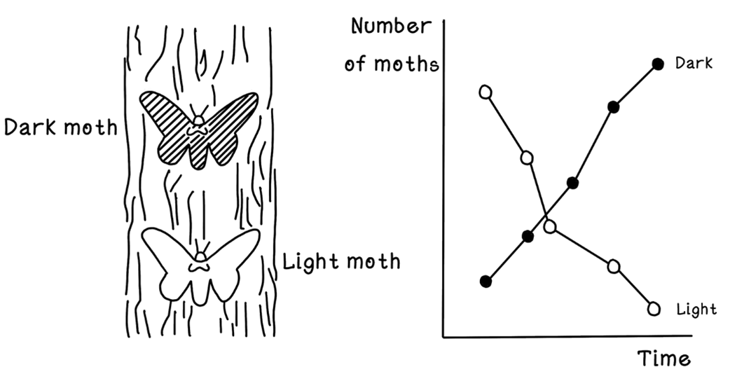
The evolution of the peppered moth
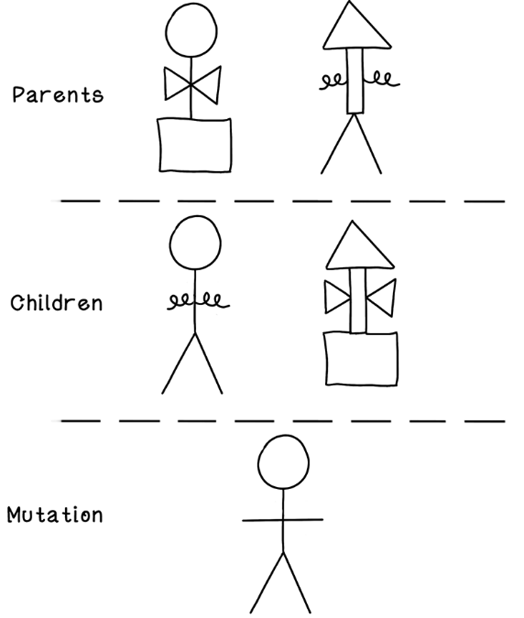
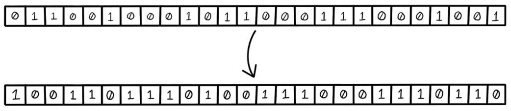
A simple example of reproduction and mutation
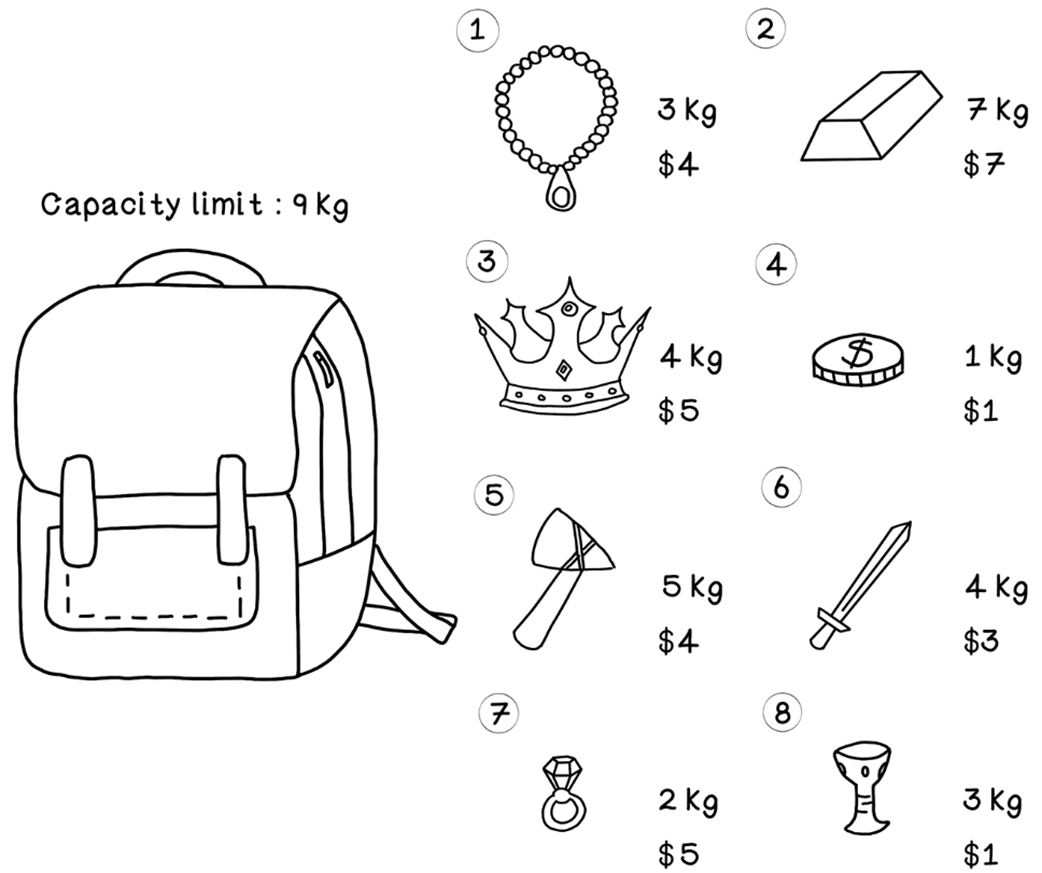
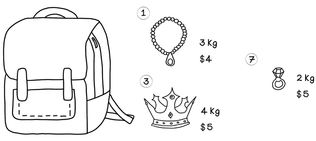
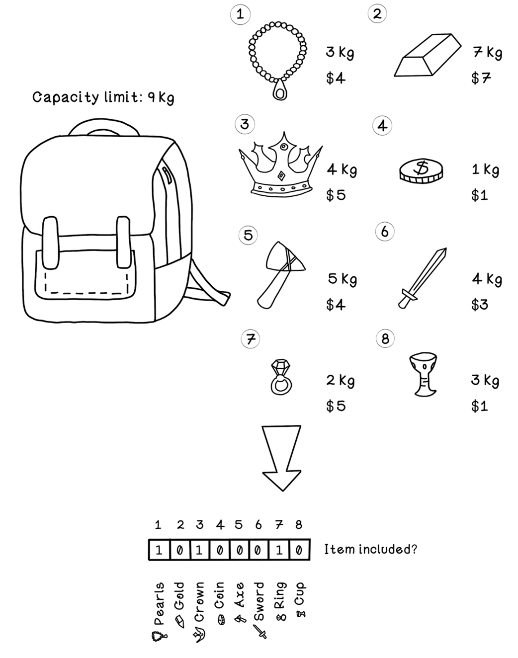
A simple Knapsack Problem example
The optimal solution for the simple Knapsack Problem example
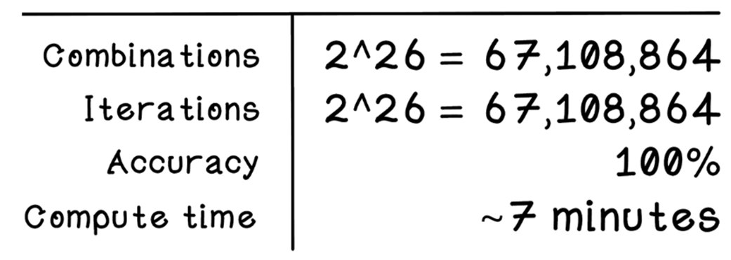
Performance analytics of brute-forcing the Knapsack Problem
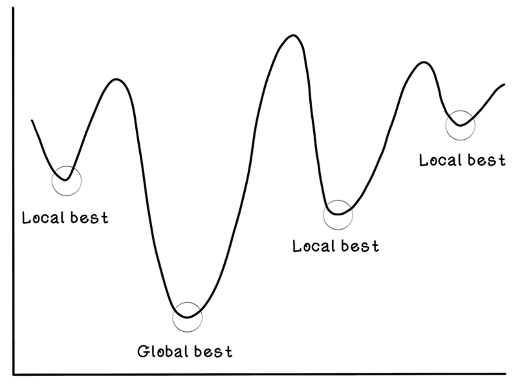
Local best vs. global best
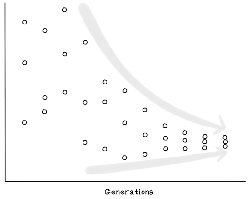
Diversity to convergence
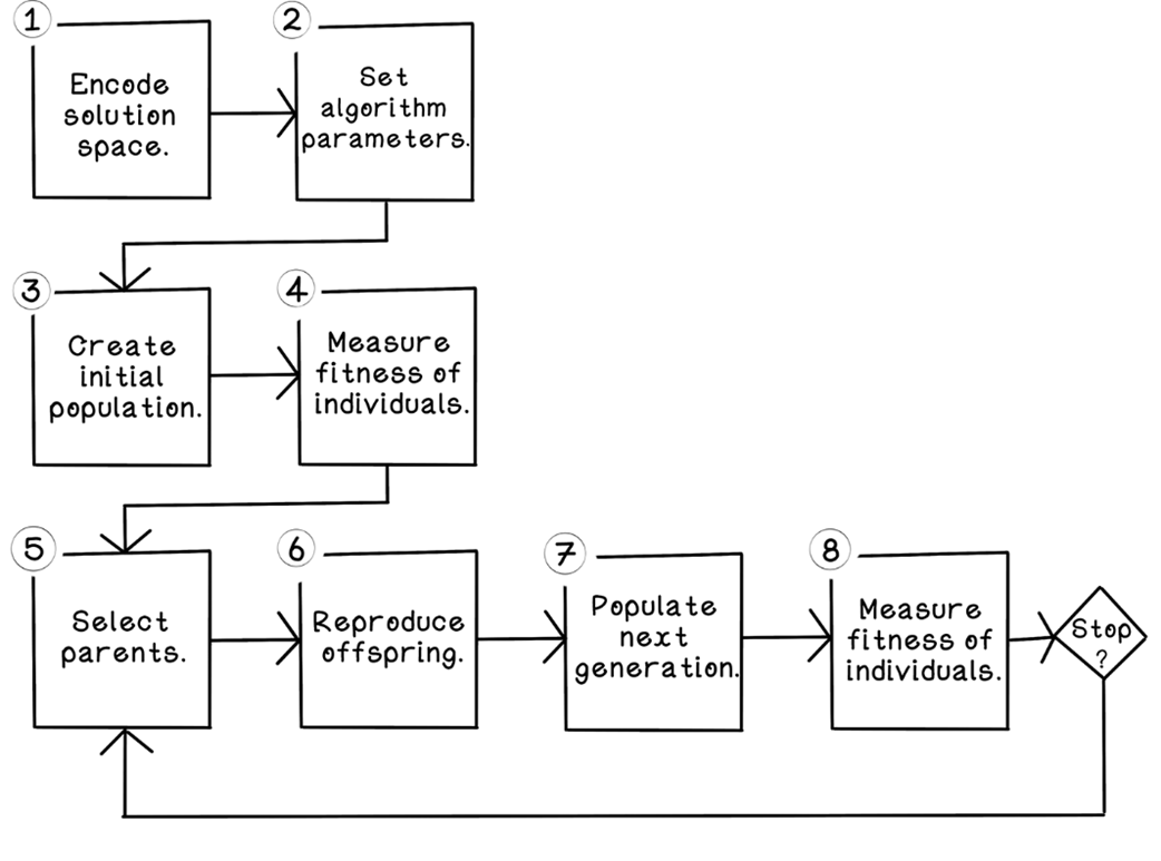
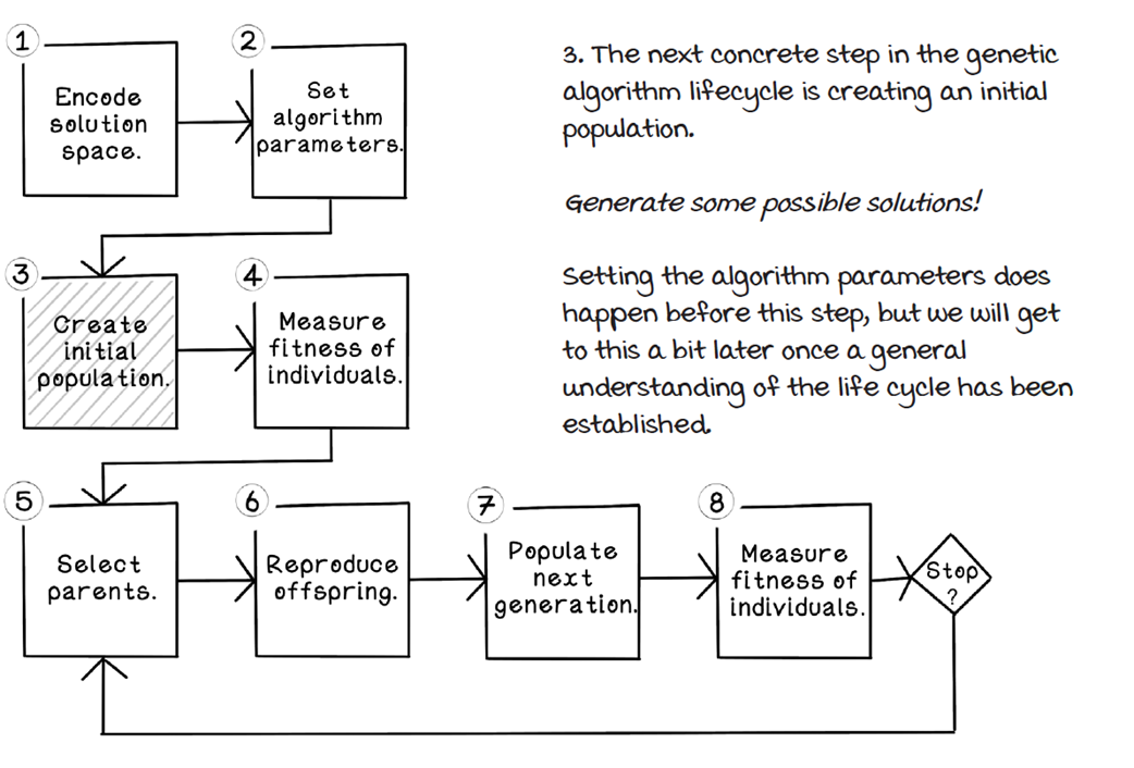
Genetic algorithm life cycle
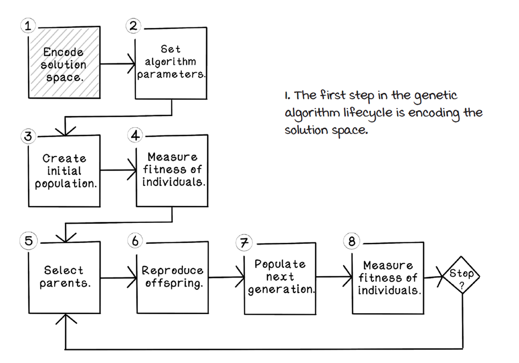
Encode the solution.
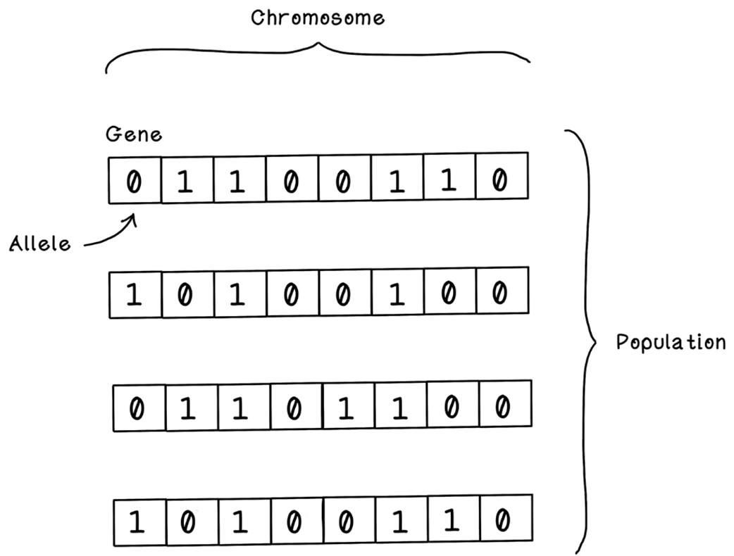
Terminology of the data structures representing a population of solutions
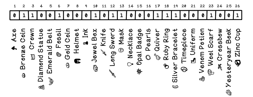
Binary-encoding the Knapsack Problem
Binary-encoding the larger dataset for the Knapsack Problem
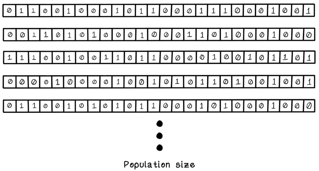
Create an initial population.
An example of a population of solutions
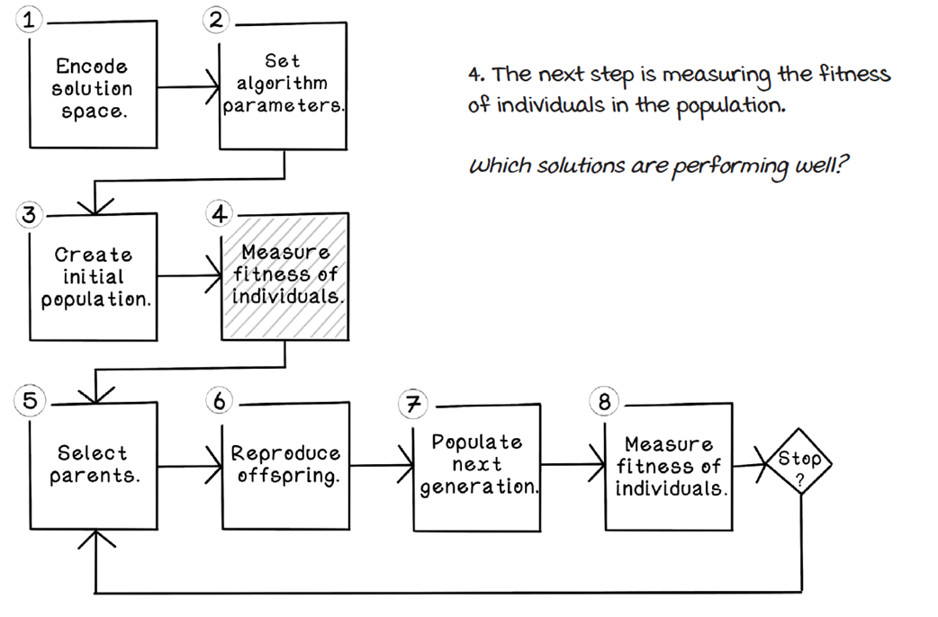
Measure the fitness of individuals.
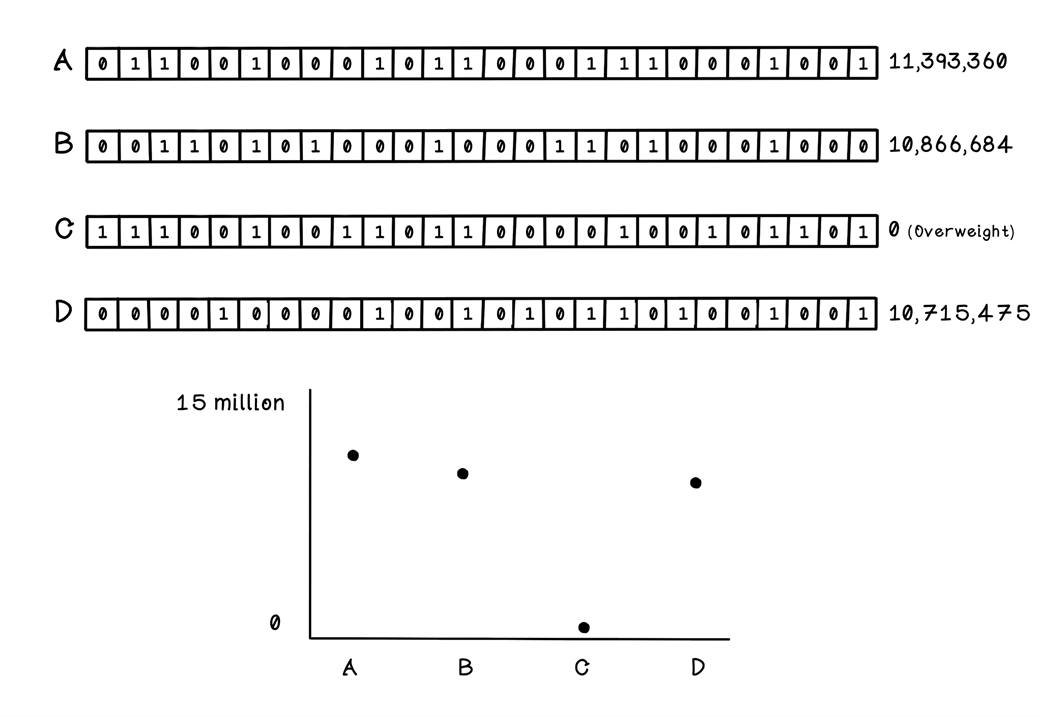
Measuring the fitness of individuals
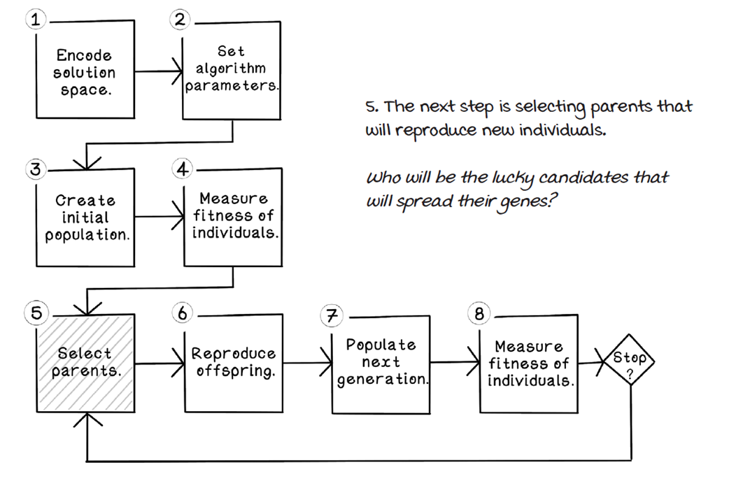
Select parents.
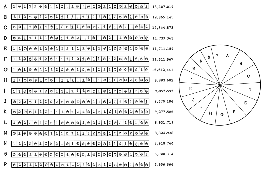
Determining the probability of selection for each individual
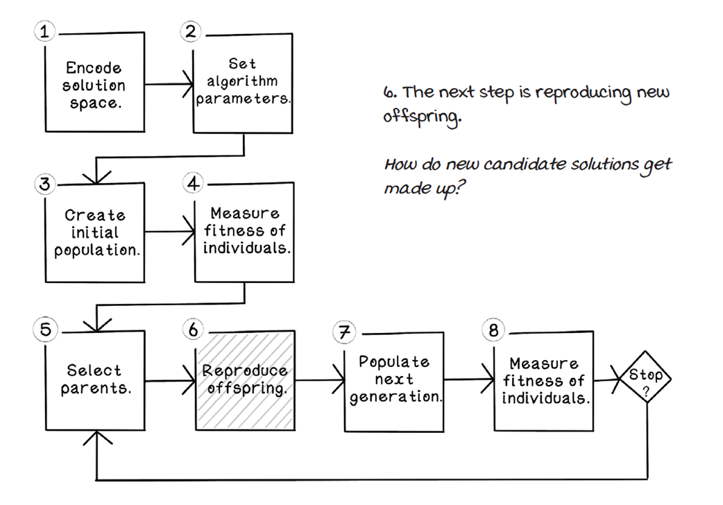
Reproduce offspring.
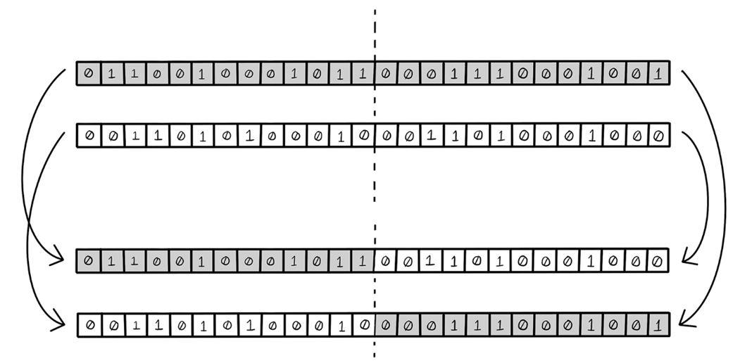
Single-point crossover
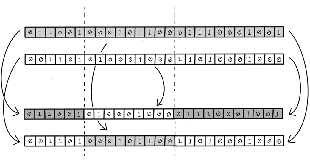
Two-point crossover
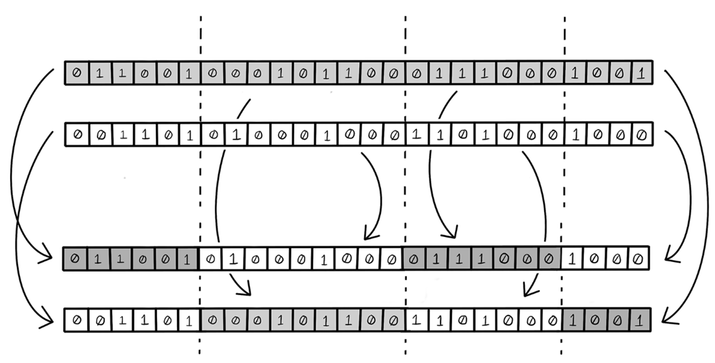
Uniform crossover
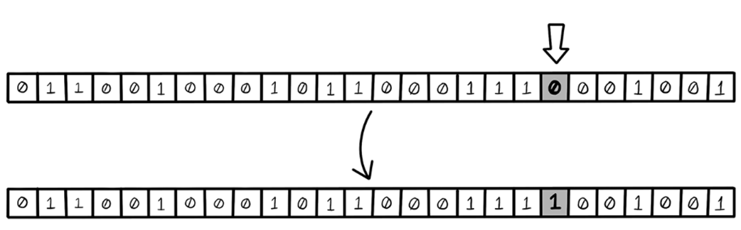
Bit-string mutation
Flip-bit mutation
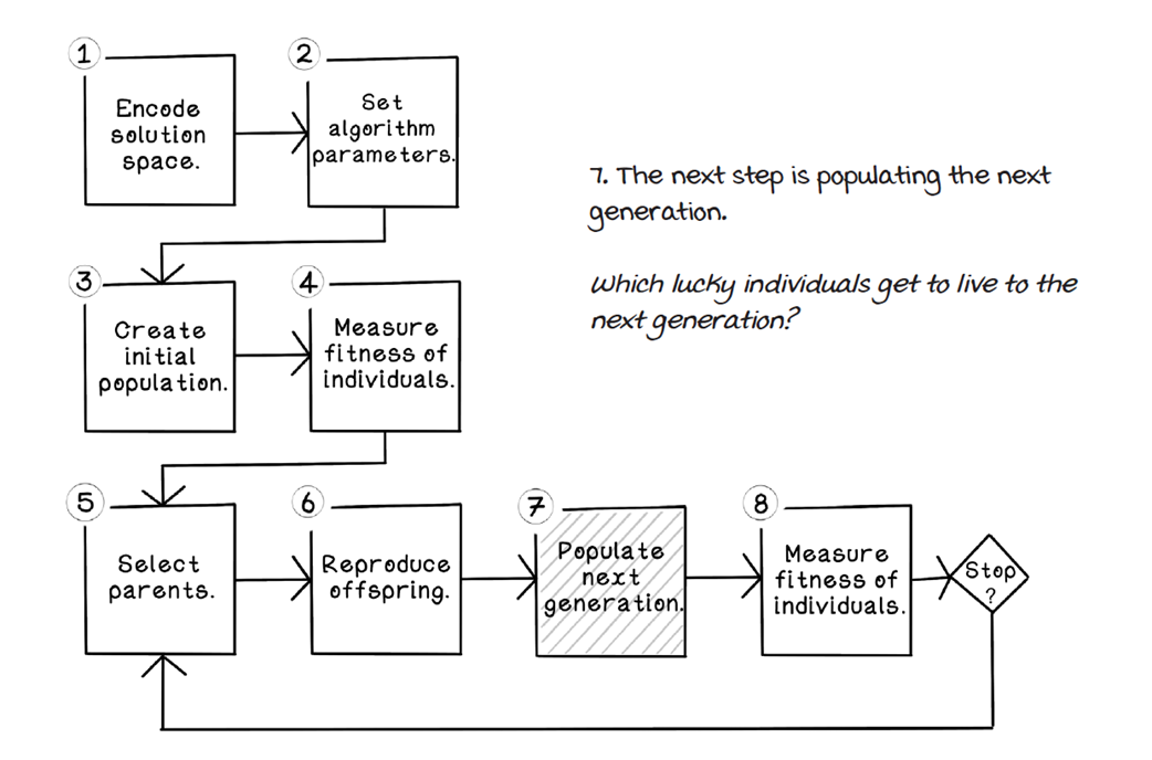
Populate the next generation.
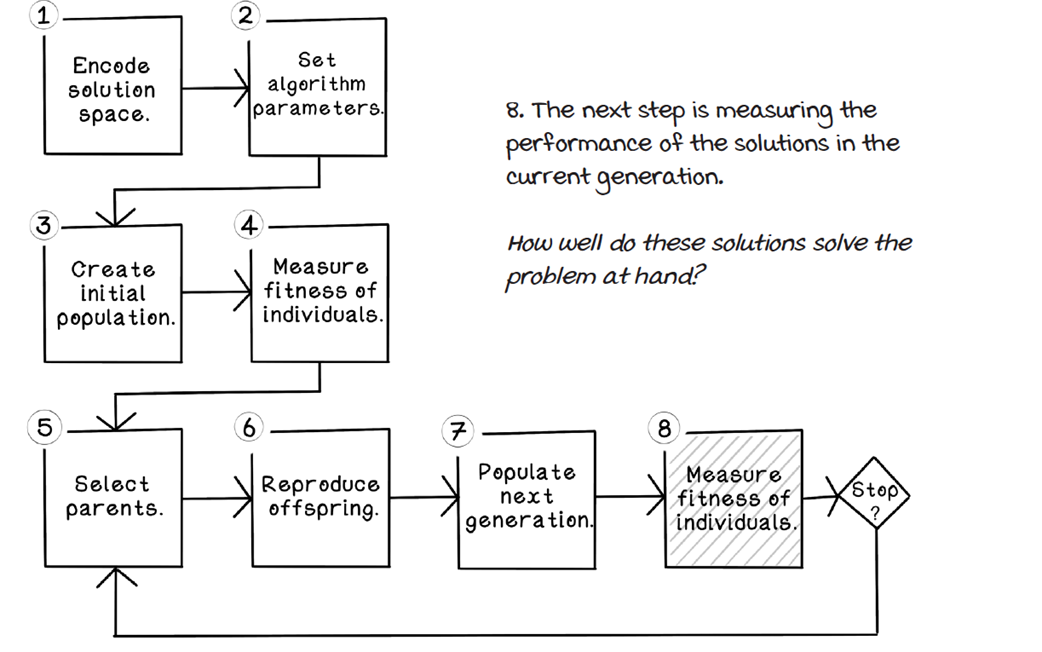
Measure the fitness of individuals.
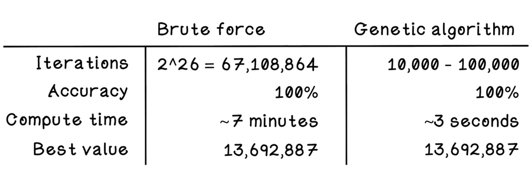
Brute-force performance vs. genetic algorithm performance
Summary of evolutionary algorithms
FAQ
What is an evolutionary algorithm, and how is it inspired by natural selection?It’s a search and optimization method that mimics biological evolution. A population of candidate solutions is created, their “fitness” is evaluated, the better ones are more likely to reproduce (selection), their information is mixed (crossover), small random changes are introduced (mutation), and this repeats over generations to discover high-quality solutions.When is a genetic algorithm a good choice compared with brute force or greedy methods?Use it for large, complex optimization spaces with many local optima where exhaustive search is infeasible and simple heuristics get stuck. It’s well-suited when “good enough” solutions are acceptable, stochastic exploration is valuable, and evaluating a candidate is cheap relative to enumerating all possibilities (for example, Knapsack variants, routing, packing, scheduling).What are the main steps in the genetic algorithm life cycle?- Create an initial, diverse population of candidates
- Evaluate fitness for each individual
- Select parents probabilistically, biased by fitness
- Reproduce via crossover and mutation to generate offspring
- Form the next generation (survivor selection)
- Repeat until a stopping condition is metHow are solutions represented, and why does encoding matter?The solution state (chromosome) is a structured representation made of genes (with allele values). Choosing the right encoding lets crossover and mutation produce valid, meaningful variations. For the Knapsack Problem, binary encoding (0 = exclude, 1 = include) is simple and efficient; other problems may need real-valued, permutation, or tree encodings.How should the initial population be generated while handling constraints?Seed diverse, random individuals but respect constraints. Two common approaches are:
- Penalties: allow invalid candidates but assign very poor fitness.
- Repair: automatically modify invalid candidates into valid ones (e.g., remove items to meet capacity).
Avoid construction bias (e.g., always filling from one side); generate full chromosomes first, then validate.How is fitness defined in the Knapsack example, and why penalize invalid solutions?Fitness is the total value of selected items while obeying the weight limit. Candidates that exceed capacity are heavily penalized (often to zero) so the algorithm learns that violating constraints is unacceptable, even if the value is high.How does roulette-wheel selection work, and what are steady-state vs. generational models?Roulette-wheel assigns each individual a probability proportional to its fitness; random draws pick parents, giving stronger candidates more chances without excluding weaker ones entirely. Population models:
- Steady-state: replace only a fraction each generation (maintains continuity).
- Generational: replace the entire population with offspring (more turnover, faster shifts).What are crossover and mutation, and when should I use different variants?- Crossover mixes parent genes:
- Single-point: split once; simple and fast.
- Two-point: swap a middle segment; adds variety.
- Uniform: use a random mask per gene; maximizes mixing.
- Mutation adds random tweaks (e.g., bit flips) to preserve diversity and escape local optima. Use higher mutation early (exploration), then lower it later (exploitation). Too much mutation erodes good solutions; too little risks stagnation.How are survivors chosen, how do we balance exploration vs. exploitation, and when do we stop?Survivor selection can be probabilistic or elitist; pure elitism risks premature convergence. Balance:
- Exploration: mutation and diverse selection to discover new regions.
- Exploitation: selection and crossover to refine good areas.
Stop after a fixed number of generations, reaching a target fitness, or detecting stagnation (little or no improvement across generations).Which parameters matter most, and what are practical use cases?Key knobs: encoding, population size, initialization, parent/survivor selection, crossover type, mutation method/rate, offspring count, and stopping criteria. Typical use cases include combinatorial optimization (knapsack, routing, packing), feature selection in ML, logistics scheduling, and problems like code breaking where exploring vast search spaces is essential.
pro $24.99 per month
access to all Manning books, MEAPs, liveVideos, liveProjects, and audiobooks!

 Grokking AI Algorithms, Second Edition ebook for free
