8 Using the quantum Fourier transform

This chapter shows how the quantum Fourier transform (QFT) and its inverse (IQFT) are used both to read out periodic structure encoded in quantum states and to efficiently prepare useful probability distributions. It connects interference patterns familiar from physics and digital signal processing to quantum computation, highlighting the discrete sinc distribution as the characteristic signature that emerges when phase information is converted into measurable magnitudes. The material motivates these tools for core tasks such as frequency extraction, sampling from structured distributions, and as building blocks for algorithms like quantum phase estimation and number-oriented applications in optimization.

The chapter first encodes a complex sinusoid (a geometric sequence state) on n qubits by applying Hadamards followed by phase rotations with angles that double across qubits, thereby embedding a frequency in relative phases. Applying the IQFT converts phase differences into magnitude differences whose envelope follows a discrete sinc pattern: integer frequencies collapse to a single outcome, while non-integers spread probability around the nearest integers, yielding what the authors call phased discrete sinc states. Several equivalent closed forms for these amplitudes are given (e.g., product-of-cosines and a sinc-ratio), periodicity is noted modulo 2^n, and a qubit-reversed implementation is provided to avoid final swaps without changing the resulting distribution.

To build intuition, the same discrete sinc probabilities are recast as a sequence of coin tosses with step-dependent biases, revealing a recursive, digit-by-digit view of the distribution. The chapter then leverages the QFT for state preparation: by seeding a few well-chosen Fourier coefficients and applying a QFT (in reversed order, without swaps), one can encode trigonometric distributions in the measurement probabilities. Examples include a raised-cosine distribution and a sin^4-based distribution, both of which serve as practical, tunable approximations to bell-shaped (normal-like) densities. These constructions illustrate how Fourier-domain design enables compact, efficient quantum circuits for sampling and downstream algorithmic use.

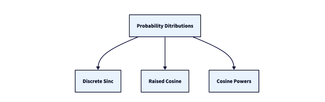
A dependency diagram of concepts covered in this chapter.

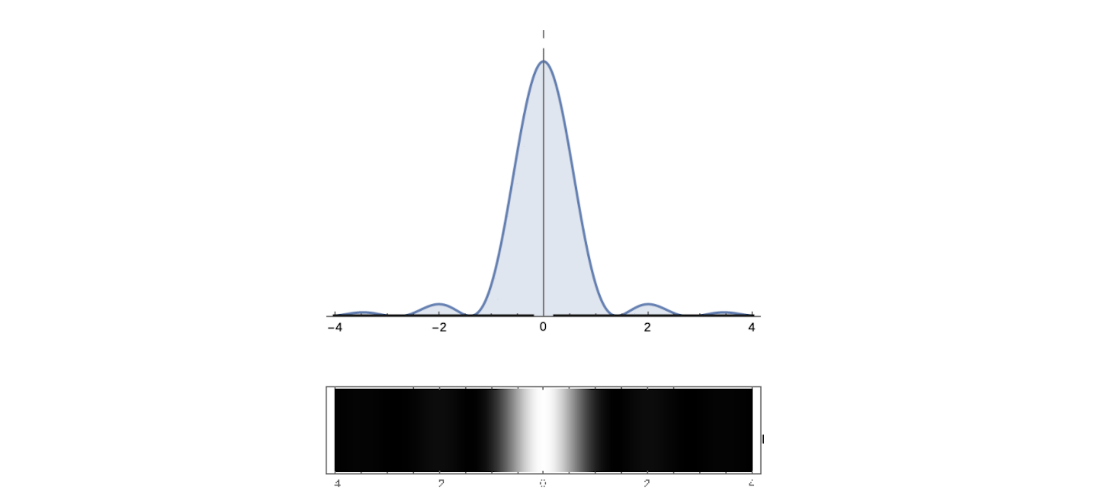
The diffraction pattern on a screen resulting from a single-slit experiment.

An example plot of diffraction intensity based on a diffraction pattern where the x-axis is the distance from the slit.

Plot of \(\text{sincd}_3\) for \(-8 \le x \le 8\).

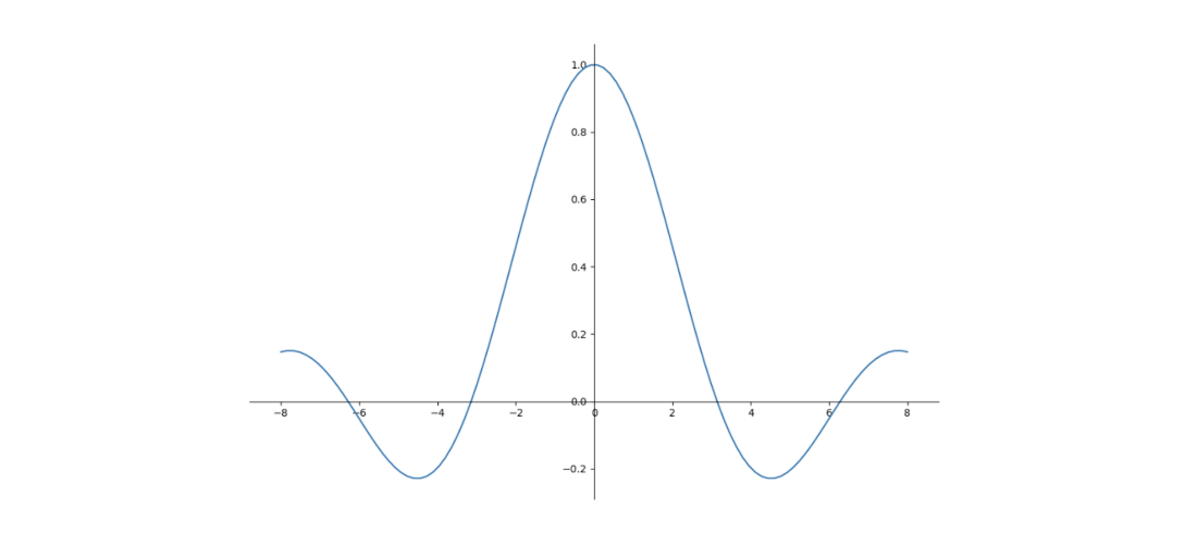
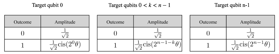
Table 8.1 An \(n\)-qubit geometric sequence state for an angle \(\theta\), where \(0 \le k < 2^n\).

The state tables of a three-qubit state after applying a Hadamard gate to each qubit, starting with the default state.

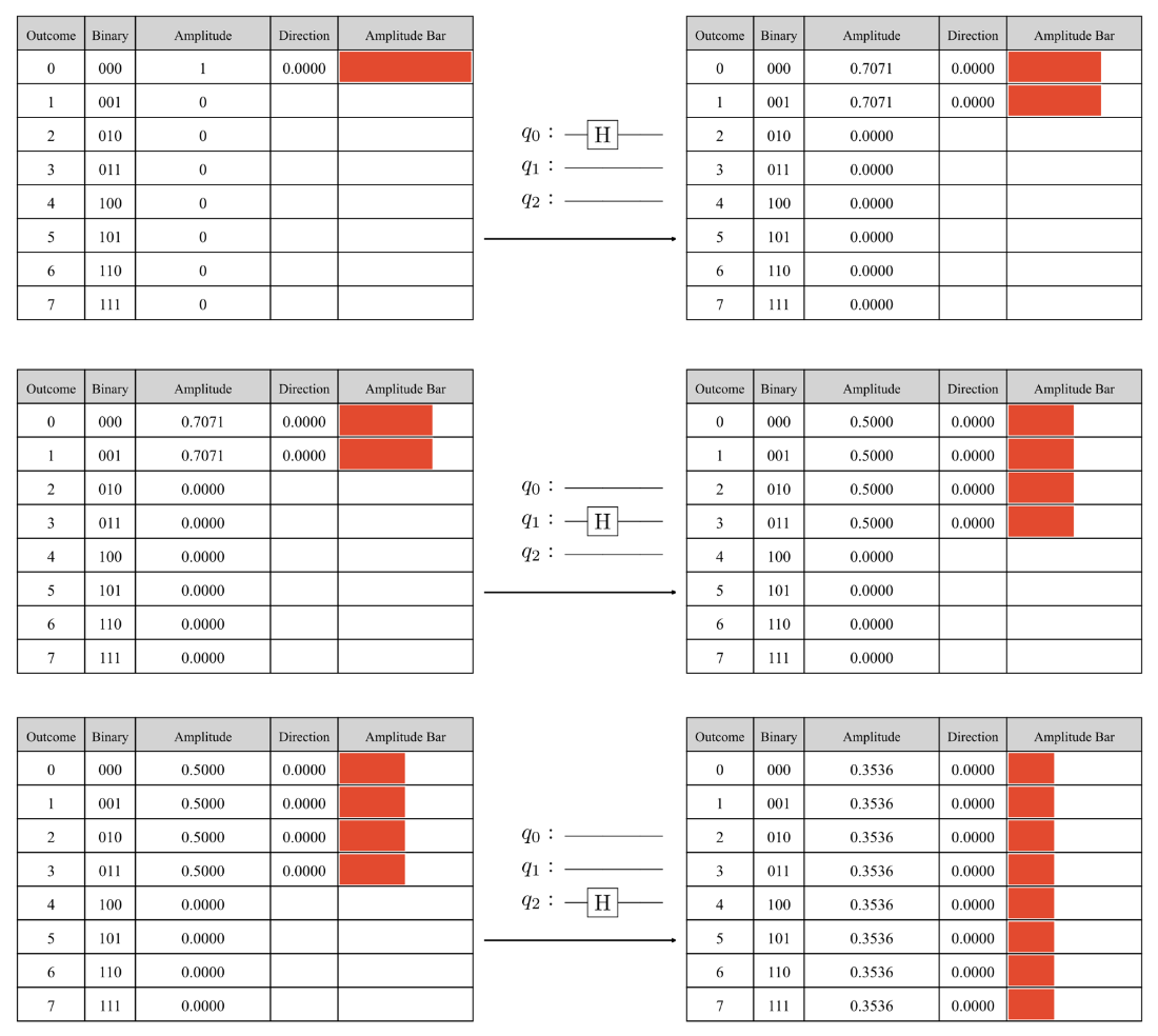
The state tables before and after applying a phase gate to target qubit 0 with angle \(\theta = \frac{\pi}{3}\).

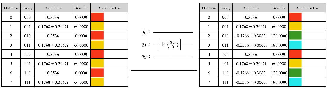
The state tables before and after applying a phase gate to target qubit 1 with angle \(2 \theta = \frac{2\pi}{3}\).

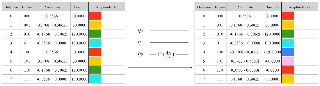
The state tables before and after applying a phase gate to target qubit 2 with angle \(4 \theta = \frac{4\pi}{3}\).

A tree diagram representation of the encoding pattern for a geometric sequence state with \(n = 3\) qubits and an angle \(\frac{\pi}{3}\).

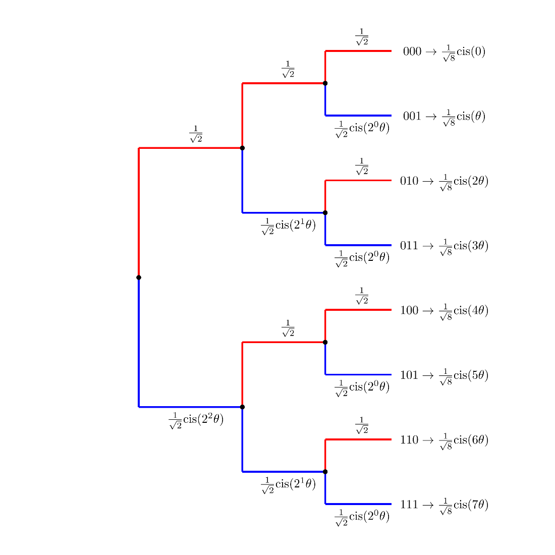
In a geometric sequence state with \(n\)-qubits and an angle \(\theta\), the amplitude corresponding to each outcome \(0 \le k < 2^n\) is the product of the factor for the target qubit digit in the binary form of the outcomes.

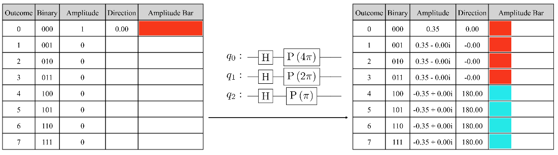
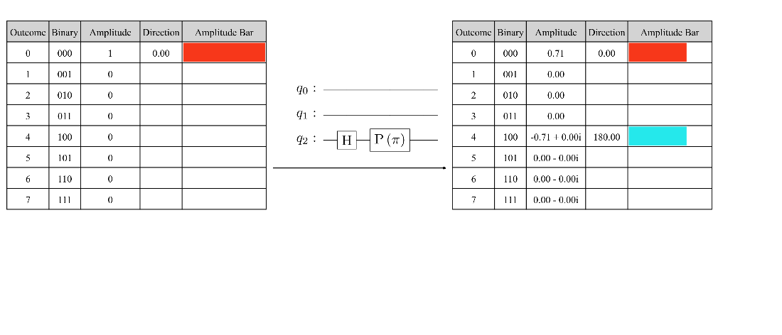
The encoding of a geometric sequence state with \(n = 3\) qubits and angle \(\theta = 4\frac{2\pi}{2^n} = \pi\), starting with the default state.

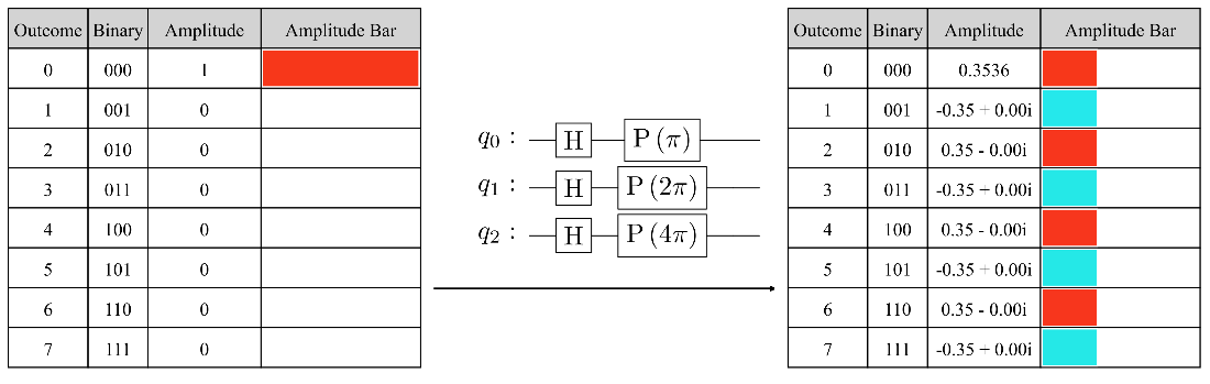
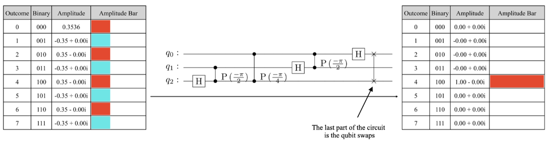
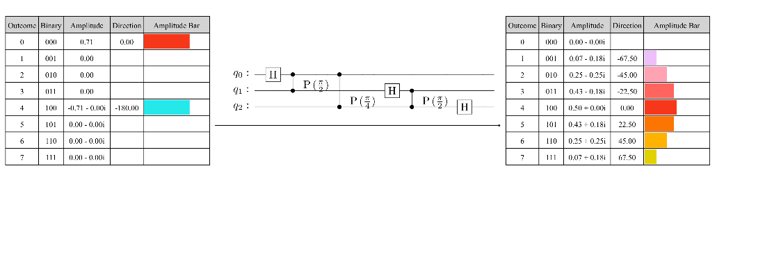
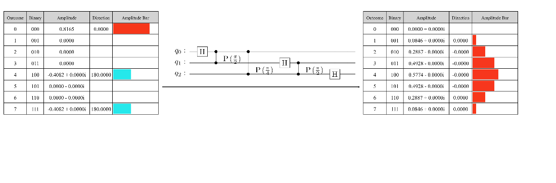
The state tables before and after applying the IQFT to the geometric sequence state with \(n = 3\) qubits and angle \(\theta = 4\frac{2\pi}{2^n} = \pi\).

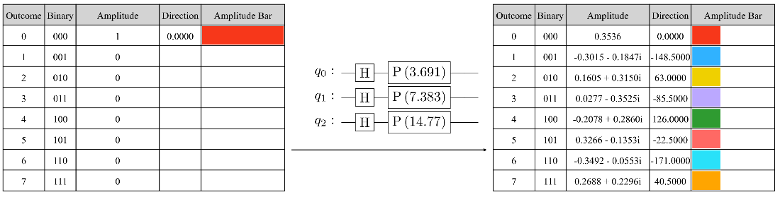
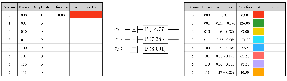
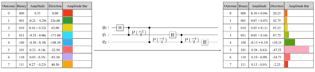
The encoding of a geometric sequence state with \(n = 3\) qubits and an angle \(\theta = 4.7\frac{2\pi}{2^n}\), starting with the default state.

The state tables before and after applying the IQFT to the geometric sequence state with \(n = 3\) qubits and an angle \(\theta = 4.7\frac{2\pi}{2^n}\).

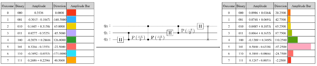
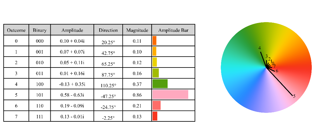
The amplitude pattern for the encoding of \(v = 4.7\) in a three-qubit state.

The amplitude pattern for the encoding of \(v = 4.3\) in a three-qubit state.

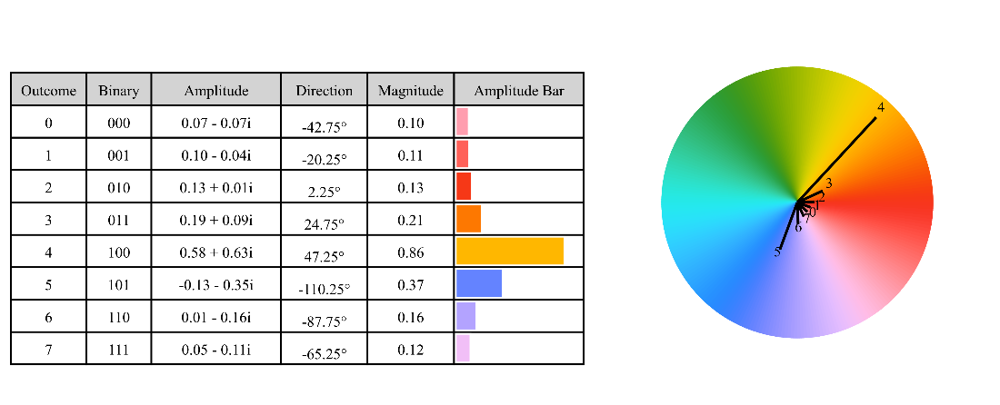
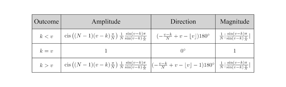
Table 8.2 The general form of a phased discrete sinc state with \(n\)-qubits, where \(0 \le k < 2^n\), and an encoded frequency \(v\), where \(0 \le v < 2^n\).

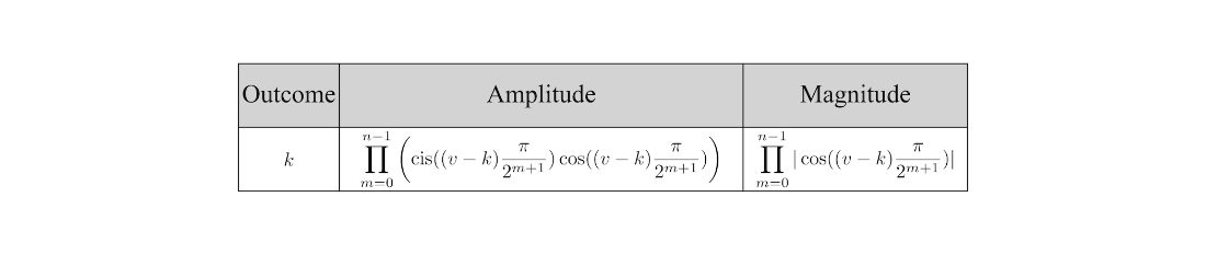
Table 8.3 The general form of a phased discrete sinc state with \(n\)-qubits, where \(0 \le k < 2^n\), and an encoded frequency \(v\), where \(0 \le v < 2^n\).

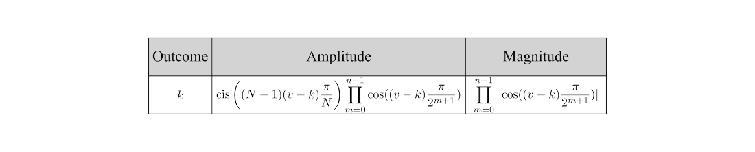
Table 8.4 The general form of a phased discrete sinc quantum state with \(n\) qubits, where \(0 \le k < 2^n\), and an encoded frequency \(v\), where \(0 \le v < 2^n\).

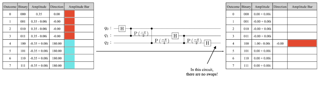
Encoding a geometric sequence state using the reverse index order with \(n = 3\) qubits and an angle \(\theta = 4\frac{2\pi}{2^n} = \pi\).

The state tables before and after applying the IQFT (without swaps).

The encoding of a geometric sequence state using the reverse index order with \(n = 3\) qubits and angle \(\theta = 4.7\frac{2\pi}{2^n}\).

The state tables before and after applying the IQFT (without swaps).

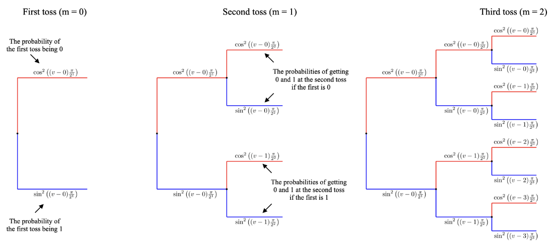
The probabilities of getting a 0 or 1 at each of the three tosses.

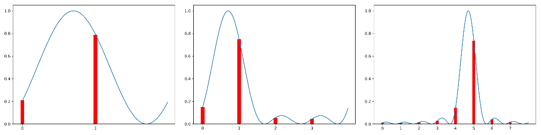
Frequency of outcomes and discrete sinc probability distribution for \(v = 4.7\) and \(n = 1\), \(n = 2\), and \(n = 3\). Note that for \(n = 1\) and \(n = 2\) the actual encoded frequency is 0.7.

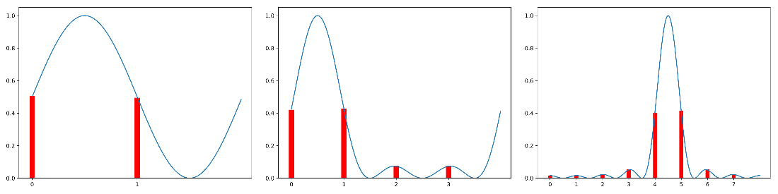
Frequency of outcomes and discrete sinc probability distribution for \(v = 4.5\) and \(n = 1\), \(n = 2\), and \(n = 3\). Note that for \(n = 1\) and \(n = 2\) the actual encoded frequency is 0.5.

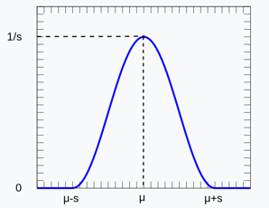
The raised cosine probability density function.

Encoding the starting frequencies for the raised cosine in the amplitudes of a three-qubit quantum state.

Applying a QFT to the qubits in a three-qubit state in reverse order (without swaps).

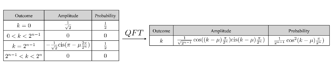
The general state tables for encoding the raised cosine probability density function for \(\mu = s = 2^{n - 1}\) in a quantum state.

The general state tables for encoding the raised cosine probability density function in a quantum state.

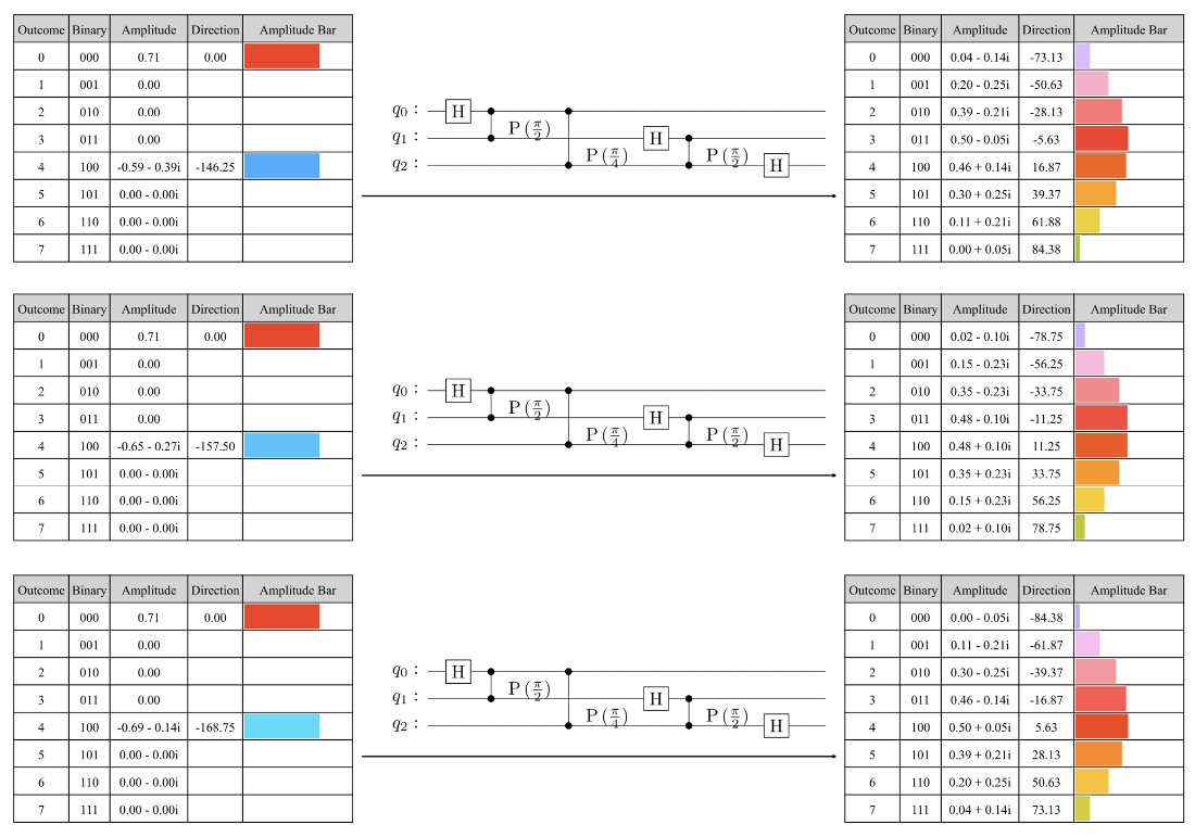
Examples of encoding the raised cosine probability density function in a three-qubit quantum state with varying \(\mu\) values.

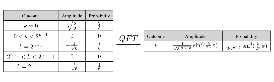
The general state tables for encoding three starting frequencies in a quantum state followed by a QFT.

Encoding three starting frequencies in the amplitudes of a three-qubit quantum state.

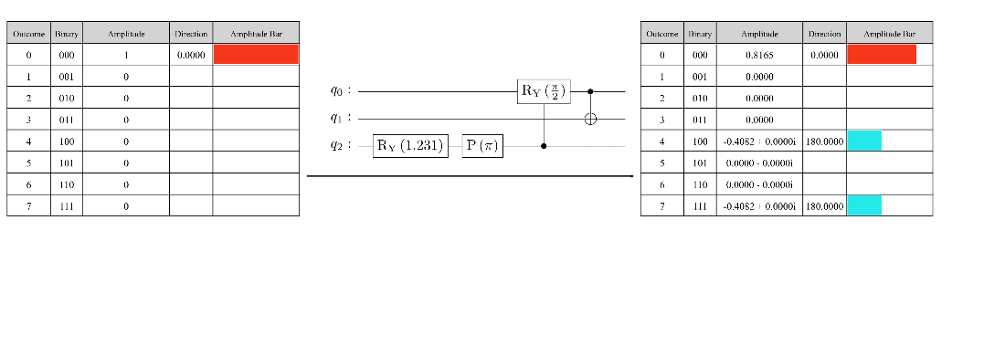
Applying a QFT to the qubits in a three-qubit quantum state in reverse order (without swaps).

• The discrete sinc function comes from the sinc function, which is very important in the field of digital signal processing.
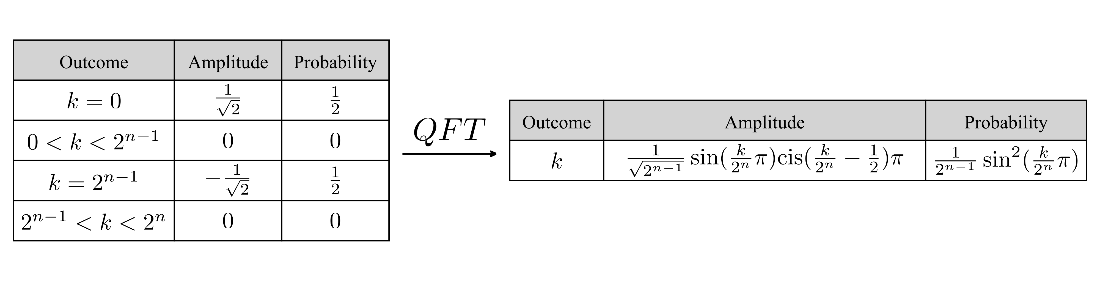
• The discrete sinc function also appears in quantum computing. Specifically, when we encode a frequency value or angle in a quantum state and then apply the IQFT, the magnitudes of the amplitudes of the resulting state match the discrete sinc function. We call a state with this pattern a phased discrete sinc state.
• We can express the general form of a phased discrete sinc state with \(n\) qubits, outcomes \(0 \le k < 2^n\), and an encoding frequency value \(v\), using the state tables below.

• We can use the phased discrete sinc state to estimate the encoded frequency value, \(v\). If \(v\) is an integer, the magnitude of the amplitude corresponding to that integer will be 1, and the rest will be 0. If \(v\) is a non-integer, it will lie between the outcomes corresponding to the top two largest magnitudes.
• Another useful application of the QFT is to encode certain probability distributions in quantum states. The normal distribution is especially difficult to encode in a quantum state, but we can use other trigonometric distributions as close approximations for the normal.
• To encode a trigonometric function like the raised cosine or \(\sin^4\) in a quantum state, we encode well-chosen starting frequencies derived from the Fourier coefficients of the function into the phase of the quantum state and then apply the QFT.

FAQ