6 Quantum search and probability estimation
This chapter introduces the second major pattern of quantum computation: searching for desired outcomes using measurement-driven techniques. It centers on Grover’s algorithm and the broader idea of amplitude (magnitude) amplification, which provide a quadratic speedup for unstructured search—reducing the number of queries from order N classically to roughly sqrt(N) quantumly. The narrative develops from intuition to practice: starting with the role of oracles that mark “good” outcomes, moving through the mechanism that boosts their amplitudes, and culminating in complete circuit constructions that realize the algorithm on a quantum simulator.
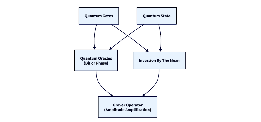
The core building blocks are phase or bit oracles that tag solutions and an inversion (often called inversion-by-the-mean) operator that reflects the state to amplify tagged amplitudes. Inner products are used to formalize similarity and guide a geometric understanding of the inversion as a reflection about a reference state. Composing an oracle O with an inversion M yields the Grover iterate G, which is applied repeatedly to rotate probability mass toward the good subspace. If the initial success probability is sin²(θ), then after j iterations it becomes sin²((2j+1)θ); choosing j near floor((π/4)√(N/L)) (with L solutions among N outcomes) maximizes the chance of measuring a good outcome, while over-iterating reduces it due to the procedure’s periodic nature.
Implementation proceeds in two layers. Classically, the chapter provides Python functions for simulating oracles, computing inner products, performing inversion, and checking the theoretical probability updates across iterations. Quantumly, it constructs circuits for the oracle (multi-controlled phase flips) and for inversion via M = A M₀ A⁻¹, where M₀ flips all amplitudes except the |0⟩ outcome and A prepares the initial state (e.g., a layer of Hadamards for uniform superposition). These pieces are assembled into a Grover iterate and then into a full Grover circuit that applies A followed by the iterate the optimal number of times, with reporting hooks to verify amplitude evolution. The chapter emphasizes that speedup depends on efficient oracles and measurement, laying groundwork for applying search and amplification across optimization and machine learning tasks.
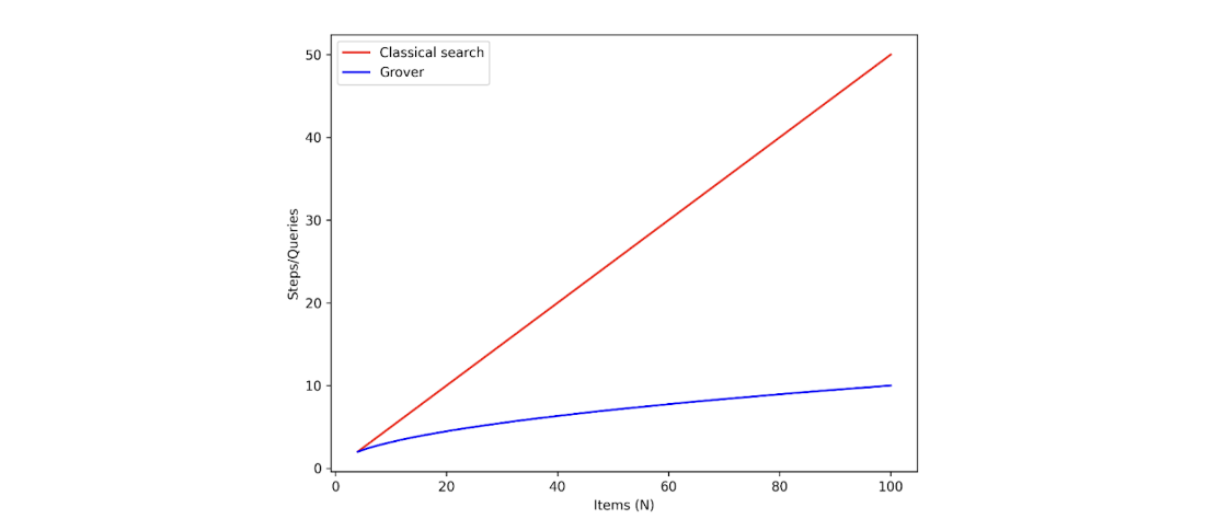
The number of steps (queries) needed to find one item in an unordered list of \(N\) items with a high probability.
A dependency diagram of concepts introduced in this chapter.
Circuit diagram of magnitude (amplitude) amplification method where operator \(A\) prepares a state and operator \(G\) is the Grover iterate.

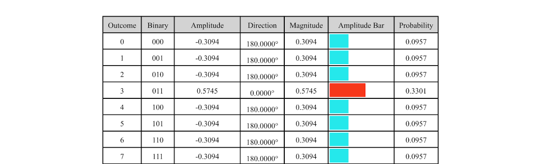
Table 6.1 A three-qubit state where all amplitudes have equal, real values.
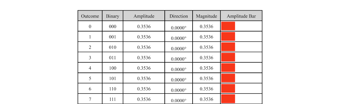
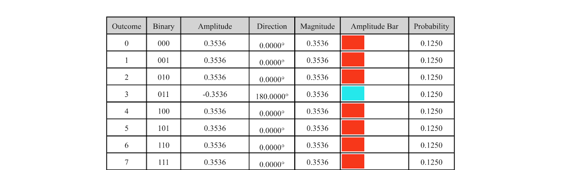
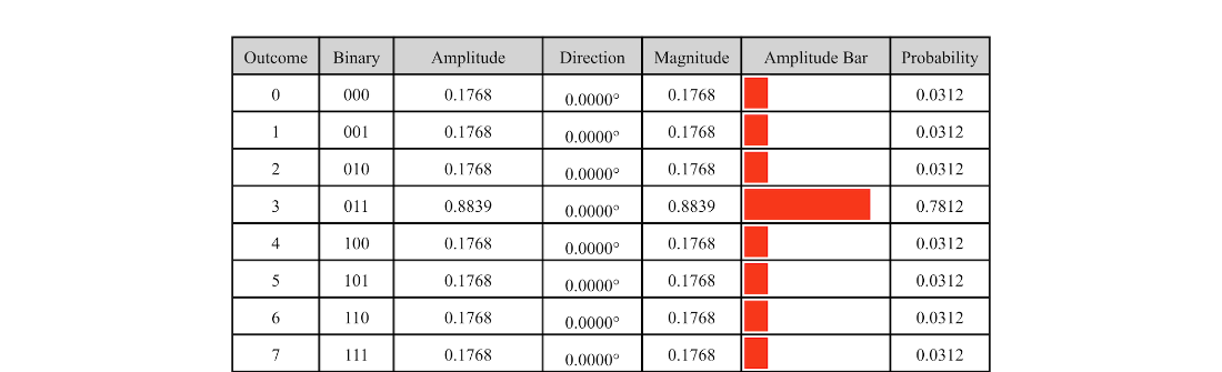
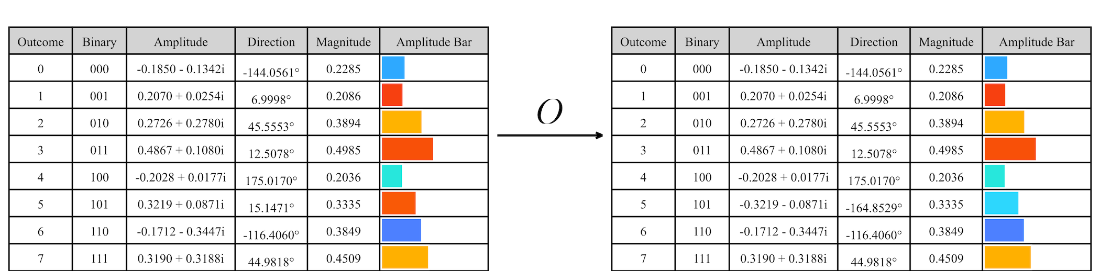
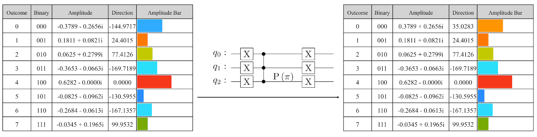
Table 6.2 A three-qubit state after a phase oracle for good outcome 3 is applied to the state in table 6.1.
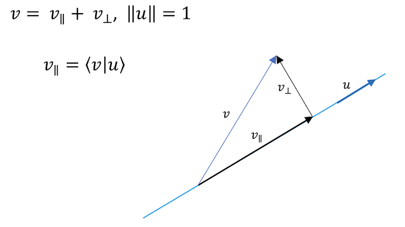
The projection of a two-dimensional vector onto another as an inner product.
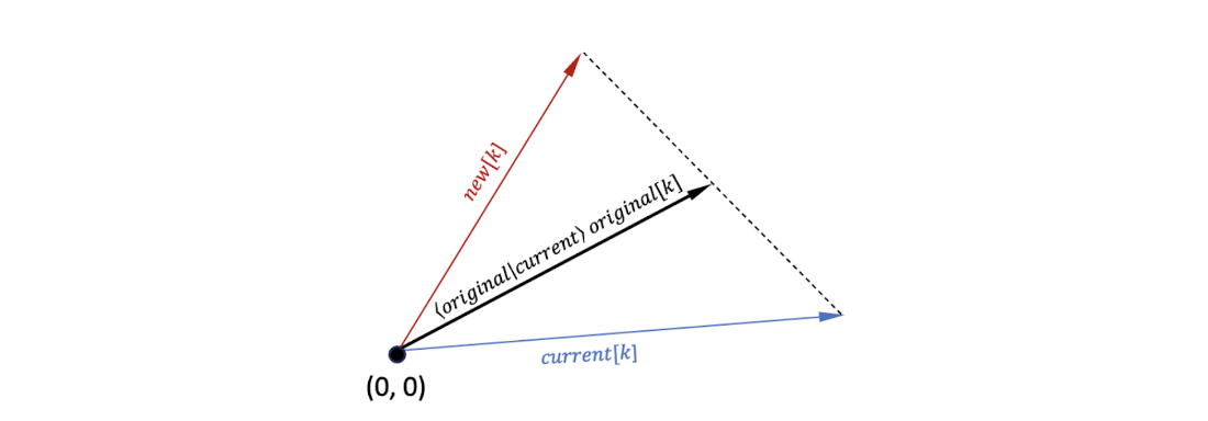
Vector visualization of the amplitudes of an outcome \(k\) before (original) and after (current) some operator is applied.

The value \(new [ k ] \) is the inversion of \(current [ k ] \) over the point \(\langle original \vert current \rangle original[k]\).
The amplitude of a bad outcome \(k\) before (\(original [ k ] \)) and after (\(current [ k ] \)) an oracle is applied.

The inversion of the amplitude corresponding to a bad outcome \(k\).

The amplitude of a good outcome \(k\) before (\(original [ k ] \)) and after (\(current [ k ] \)) an oracle is applied.

The inversion of the amplitude corresponding to a good outcome \(k\).
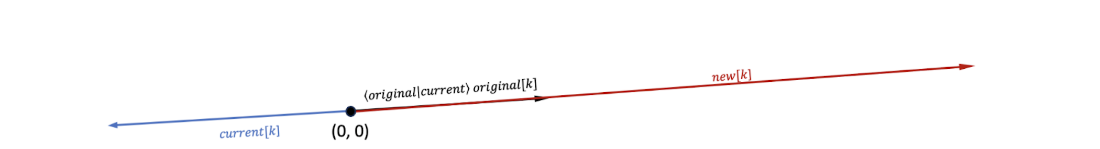
Table 6.3 The three-qubit state in table 6.2 after applying the inversion operator \(M_s\).
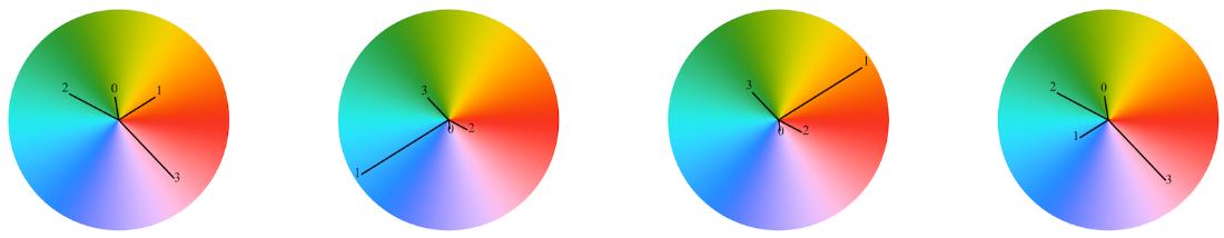
A random \(n = 3\) qubit state before and after an oracle for good outcomes 5 is applied.
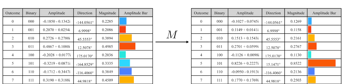
Applying the inversion operator to a random \(n = 3\) qubit state with good outcome 5.
Circuit diagram of the magnitude amplification procedure \(G^jA\) where \(G\) consists of an oracle \(O\) and the inversion operator \(M\).

The combined measurement probabilities of good and bad outcomes before and after \(j\) applications of the Grover iterate.
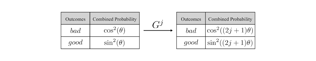
Table 6.4 A three-qubit state with good outcome 3 after applying operator \(A\) and one Grover iteration.

Table 6.5 A three-qubit state with good outcome 3 after applying operator \(A\) and two Grover iterations.
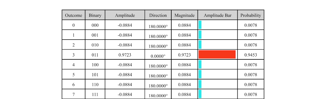
Table 6.6 A three-qubit state with good outcome 3 after applying operator \(A\) and three Grover iterations.
A random two-qubit state with good outcome 1, and the state after 1, 2, and three Grover iterations.
Circuit diagram for the magnitude amplification procedure \(G^jA\) where the operator \(G\) consists of an oracle \(O\) and the inversion operator \(M = AM_0A^{-1}\).

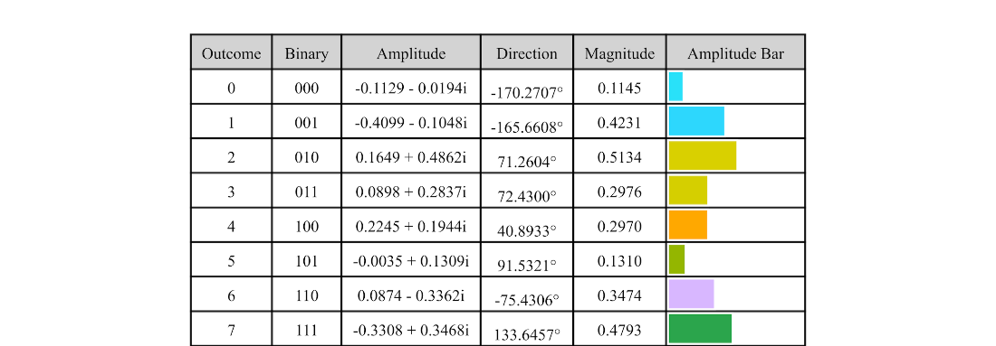
Table 6.7 A three-qubit state after applying a random operator \(A\).
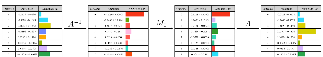
Application of the operator \(M = A M_0 A^{-1}\) to a three-qubit state prepared with a random operator \(A\), followed by the application of an oracle \(O\) for the good outcome 3.
Circuit diagram of magnitude (amplitude) amplification.

Circuit \(M_0\) for three qubits.

Applying operator \(M_0\) to a random three-qubit state.
Circuit diagram of the magnitude amplification procedure \(G^jA\) where the operator \(G\) consists of an oracle \(O\) and the inversion operator \(M = AM_0A^{-1}\).

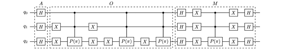
The quantum circuit for three qubits and good outcomes 1, 3, and 7.
Summary
- We can use magnitude (amplitude) amplification to increase the probability of finding one or more "good" outcomes upon measurement. This procedure can be expressed as \(G^jA\) for an integer \(j > 0\), where \(A\) is an operator that prepares a starting state and \(G\) is the Grover iterate. The operator \(G\) consists of a quantum oracle and an inversion operator.
- After \(j \ge 0\) applications of the Grover iterate, the combined measurement probability of the good outcomes is
- For \(n\) qubits (\(N = 2^n\)), and \(L\) good outcomes, the optimal number of Grover iterations (\(j\)) is
FAQ
What problem does Grover’s algorithm solve and how much speedup does it offer?
Grover’s algorithm addresses unstructured search: finding one (or more) desired item(s) among N possibilities using an oracle that tests candidates. Classically, you need about N/2 oracle calls on average; Grover’s algorithm boosts the success probability via amplitude amplification and needs about sqrt(N) oracle calls to reach a high success probability, giving a quadratic speedup.What is amplitude (magnitude) amplification and what are its main steps?
Amplitude amplification increases the measurement probability of “good” outcomes tagged by an oracle. The standard two-step pattern is: (1) Prepare an initial state with a circuit A. (2) Apply the Grover iterate G repeatedly, j times. The iterate G is the composition of the oracle O (phase-flip on good states) and an inversion (reflection) operator M about the prepared state. After j applications, good-outcome probability becomes sin^2((2j+1)θ), where sin^2(θ) is the initial success probability.What is a quantum oracle and which type is used here?
An oracle tags good outcomes. Two common kinds are: (1) Phase oracles: multiply amplitudes of good outcomes by -1. (2) Bit oracles: entangle good outcomes with an ancilla qubit that flips to 1. This chapter uses phase oracles (e.g.,phase_oracle_match(n, items)) to apply a -1 phase to specified computational-basis states.How does the inversion operator work intuitively and classically?
The inversion (often called “inversion by the mean” in the uniform case) reflects the current state about the initial state prepared by A. Classically, ifproj = ⟨original, current⟩, each amplitude is updated via current[k] = 2*proj*original[k] - current[k]. Intuitively, you mirror each amplitude around its projection onto the original state. When the original state is the uniform superposition, the reflection is around the mean amplitude, hence the name.How is the inversion implemented in a quantum circuit (the AM0A⁻¹ construction)?
Directly computing means is not quantum-friendly. Instead, you realize the reflection about A|0…0⟩ by conjugating a simple “zero-state phase flip”: - Build M0 to apply a -1 phase to outcome 0 (|0…0⟩). - Define M = A M0 A⁻¹, which reflects about the state prepared by A. Up to a global phase, this equals the diffusion operator used in Grover search. In code, M0 is built with X gates to target |0…0⟩ and a multi-controlled phase of π, then X gates again.How many Grover iterations should I run?
The optimal number of iterations is approximately floor((π/4)*sqrt(N/L)), where N = 2^n is the total number of outcomes and L is the number of good outcomes. Let sin^2(θ) = L/N. After j iterations, the success probability is sin^2((2j+1)θ). If you over-iterate, the probability starts decreasing (over-rotation), so using the optimal j is important.What role does the inner product play in amplitude amplification?
The inner product measures similarity between state vectors. In the classical inversion formula,proj = ⟨original, current⟩ is a complex scalar with magnitude at most 1; it scales/rotates the original amplitudes to define the reflection point for each component. For normalized quantum states, ⟨ψ, ψ⟩ = 1, and the projection value evolves predictably during Grover iterations (e.g., ⟨A|state after j⟩ = cos(2jθ)).How do I assemble the full Grover circuit in code?
Build three pieces: (1) A: an initializer (e.g.,uniform(n) applies H on each qubit). (2) O: a phase oracle (e.g., phase_oracle_match(n, items)) that flips marked states’ phases. (3) G: the Grover iterate constructed as grover_iterate_circuit(A, O), which appends O then the inversion circuit inversion_circuit(A) (i.e., A⁻¹, M0, then A). Use grover_circuit(A, O, iterations) to apply A once and G repeatedly. Building Quantum Software with Python ebook for free