4 Quantum state and circuits: beyond one qubit

This chapter extends the single‑qubit foundations to multi‑qubit quantum computing, focusing on how to represent, evolve, and measure quantum states and how to express computations as circuits in Python. It introduces multi‑qubit state tables and the state vector view (a list of complex amplitudes), explains how measurement produces bitstrings whose frequencies reflect underlying probabilities, and revisits common computation patterns such as sampling, searching, and probability estimation. With these concepts in place, the chapter builds a hands‑on simulator, then demonstrates how to prepare useful states and distributions (uniform, binomial) and create quintessential entangled states (Bell states), all culminating in circuit‑level abstractions with registers and gate sequences.

Technically, an n‑qubit state is encoded as 2^n complex amplitudes whose squared magnitudes sum to one; probabilities and phases can be interconverted with amplitudes for analysis or construction. The chapter contrasts product states with entangled states and proves why Bell states cannot be decomposed into independent single‑qubit states. Gate actions are shown to recombine pairs of amplitudes that differ only in the target qubit’s bit, with efficient pair selection derived from binary indexing and “chunking.” A compact Python simulator validates states, initializes |0…0⟩, and applies gates via pairwise updates; controlled and multi‑controlled variants restrict which pairs are affected. Using these tools, the chapter prepares a uniform distribution by applying Hadamards to all qubits and encodes a binomial distribution by applying Ry rotations (with grouping by Hamming weight to match binomial counts), illustrating both amplitude design and probability shaping.

On top of these primitives, the chapter introduces circuit abstractions that mirror a common quantum SDK interface: quantum registers to index qubits and a circuit object that records transformations (x, h, ry, cx, mcx), executes them on a state, and supports measurement with repeated sampling to produce counts. Worked examples include simple multi‑qubit circuits, controlled operations, construction of Bell states, and measurement workflows that confirm theoretical probabilities. Throughout, the text emphasizes the trade‑offs between true quantum parallelism and classical simulation (where cost doubles with each added qubit), while highlighting the pedagogical advantage of simulators: full visibility into amplitudes, precise state preparation, and a smooth path from conceptual understanding to executable circuits used in later chapters.

A dependency diagram of concepts introduced in this chapter.

Table 4.1 The general form af a two-qubit state.

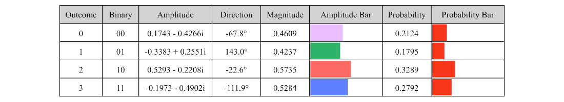
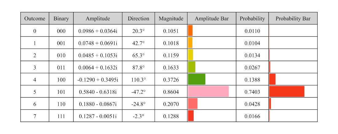
Table 4.2 The state table for a random two-qubit quantum state.

State tables for two single-qubit states.

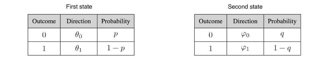
Table 4.3 State table for the product state of the two single-qubit states in figure 4.2.

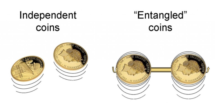
We can think of two coins with independent bias as a product state and two dependent coins as a non-product state.

State tables for first two Bell states.

State tables for last two Bell states.

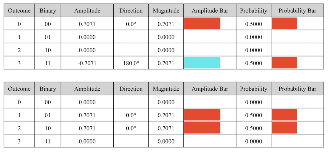
Table 4.4 The amplitudes of an \(n\)-qubit quantum state where \(0\le k < 2^n\).

Table 4.5 The probabilities and directions of a quantum state with \(n\) qubits where \(0\le k < 2^n\).

Table 4.6 The amplitudes of an \(n\)-qubit quantum state where \(0\le k < 2^n\).

Table 4.7 Table comprehension for quantum state with \(n\) qubits where \(0\le k < 2^n\).

Table 4.8 Table comprehension for quantum state with \(n\) qubits where \(0\le k < 2^n\).

Table 4.9 Table comprehension for quantum state with \(n\) qubits where \(0\le k < 2^n\).

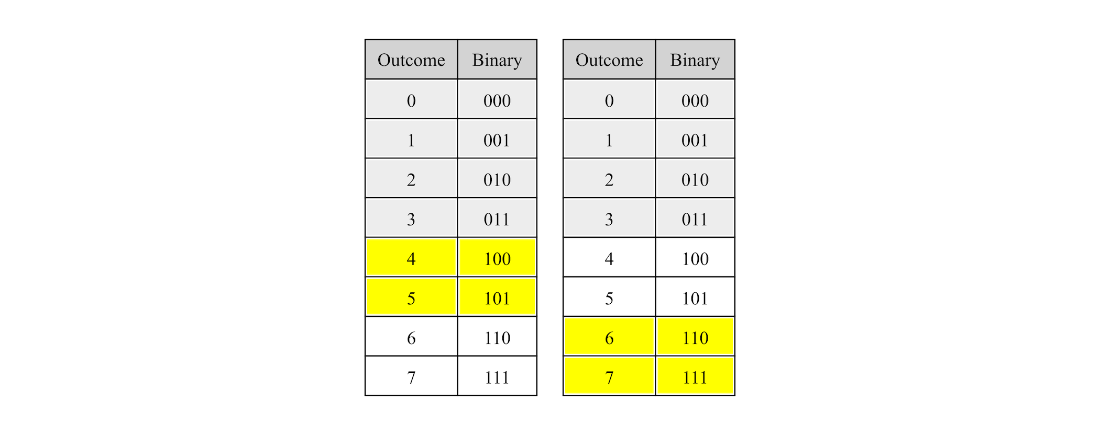
The pairs of outcomes for applying a single-qubit gate to a three-qubit system with target qubit in position 0.

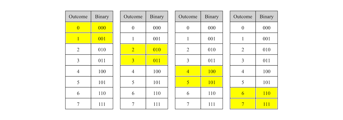
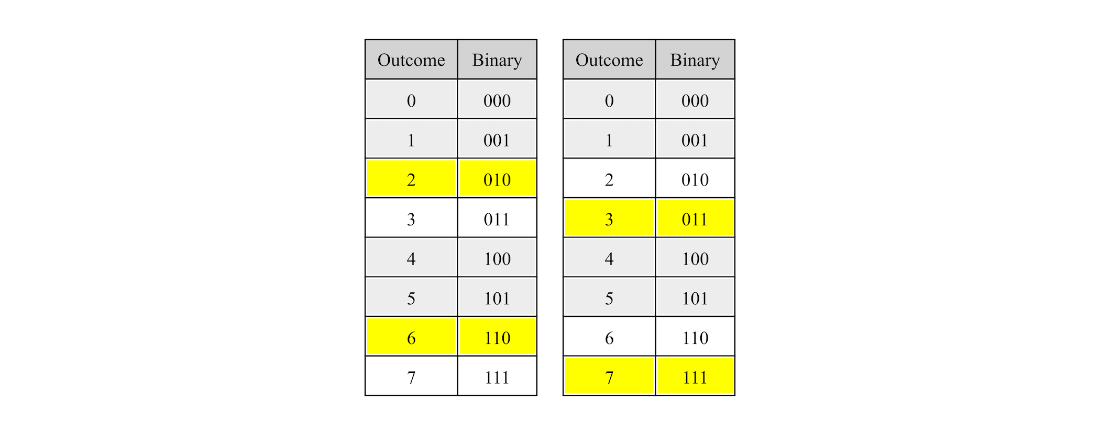
The pairs of outcomes for applying a single-qubit gate to a three-qubit system with target qubit in position 1.

The pairs of outcomes for applying a single-qubit gate to a three-qubit system with target qubit in position 2.

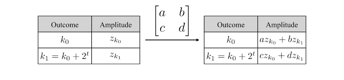
The pairs of outcomes and amplitudes of an \(n\)-qubit state (where \(0\le k < 2^n\)) before and after applying a gate transformation to target qubit \(t\).

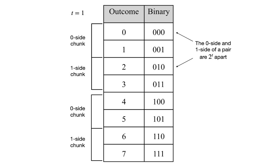
Pair generating strategy using chunks of outcomes for a three-qubit system and target qubit \(t = 1\).

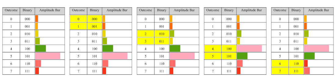
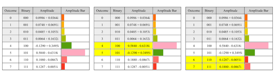
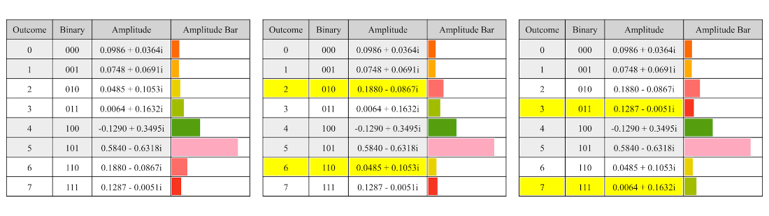
Amplitude pair processing for the X-gate applied to target qubit 0 in a three-qubit system.

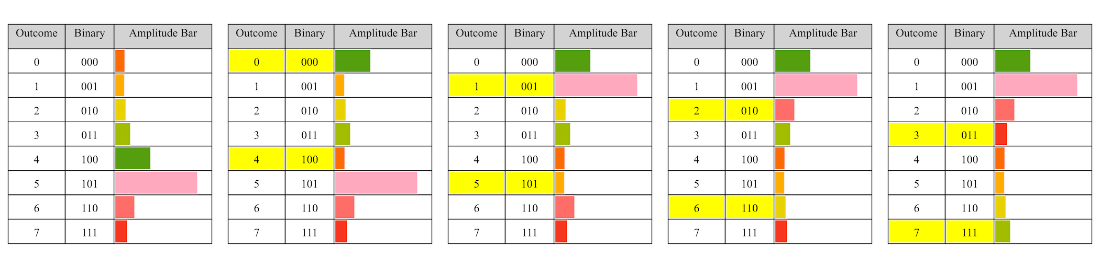
Amplitude pair processing for the X-gate applied to target qubit 2 in a three-qubit system.

Butterfly diagrams of the pairs of outcomes in a three-qubit system for targets 0, 1 and 2.

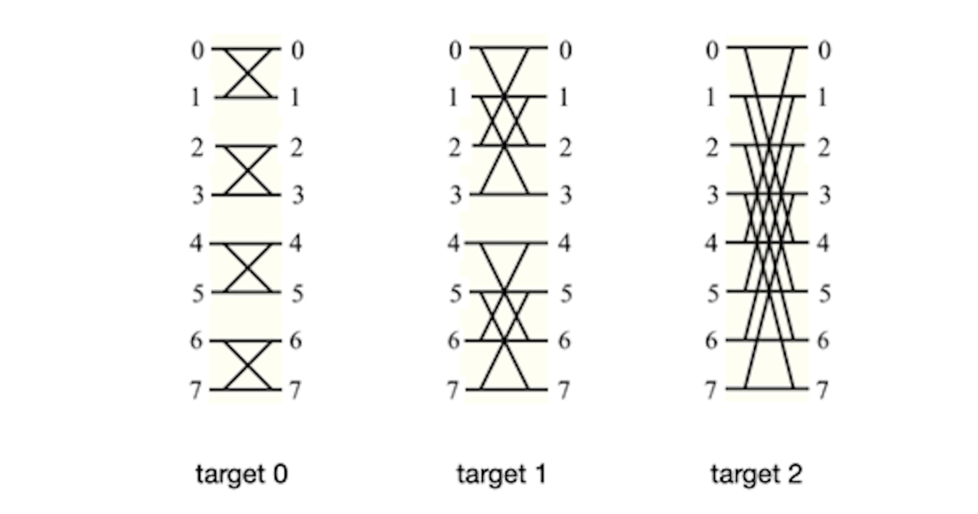
Butterfly diagrams of the pairs of outcomes in a three-qubit system for targets 0, 1 and 2.

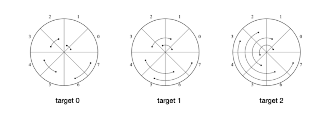
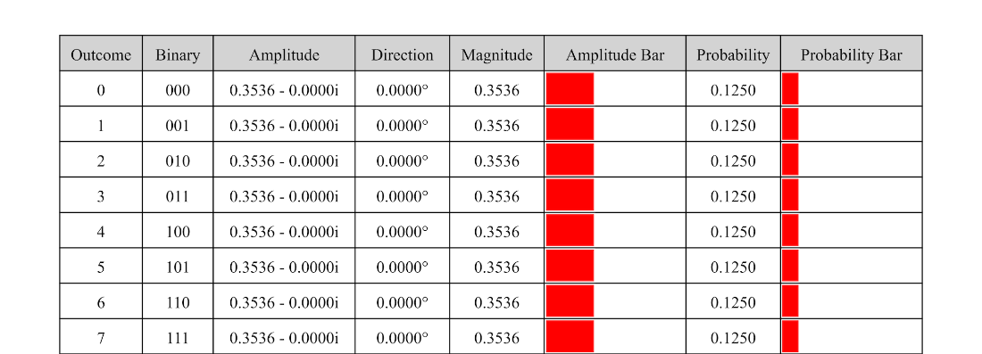
Table 4.10 The state table for the uniform probability distribution on eight outcomes.

The pairs of outcomes for applying a controlled single-qubit gate to a three-qubit system with target qubit 0 with control qubit 2.

The pairs of outcomes for applying a controlled single-qubit gate to a three-qubit system with target qubit 2 with control qubit 1.

Pair processing for applying a controlled X-gate to a three-qubit state with target qubit 0 and control qubit 2.

Pair processing for applying a controlled X-gate to a three-qubit state with target qubit 2 and control qubit 1.

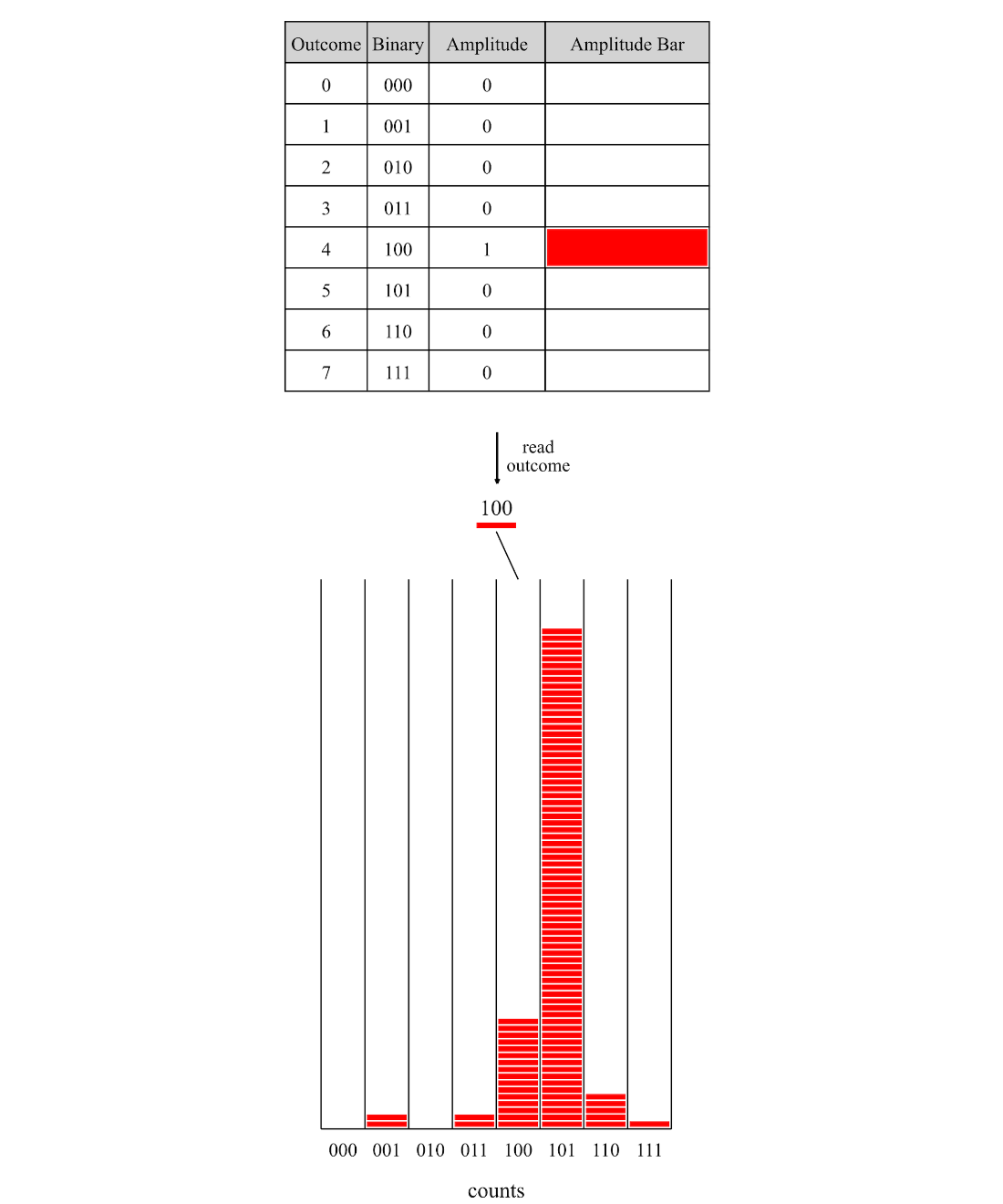
One measurement and the counts of previous measurement outcomes.

A simple three-qubit circuit.

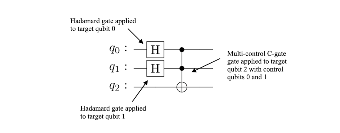
Table 4.11 The state table after applying our simple circuit.

Circuit for encoding a uniform distribution in a three-qubit state.

Table 4.12 The state table for the uniform probability distribution on eight outcomes.

The quantum circuit that applies an \(R_Y(\pi/3)\)-rotation to all three qubits of the system.

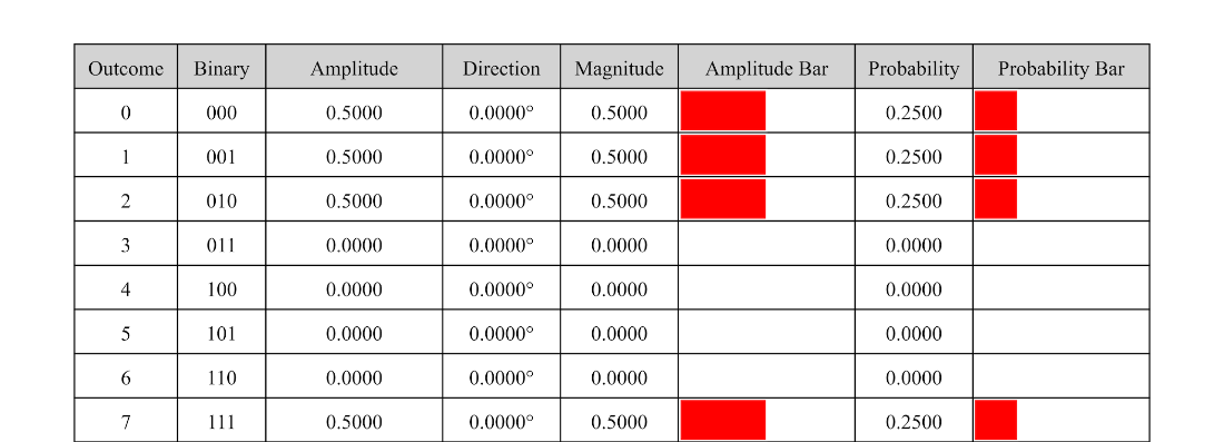
Table 4.13 The three-qubit state prepared by applying \(R_Y(\pi/3)\) gates to every qubit.

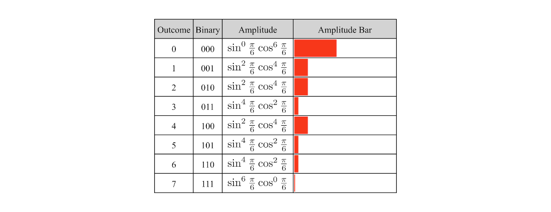
Table 4.14 The binomial distributions for \(p = \cos^2\frac{\pi}{3}\).

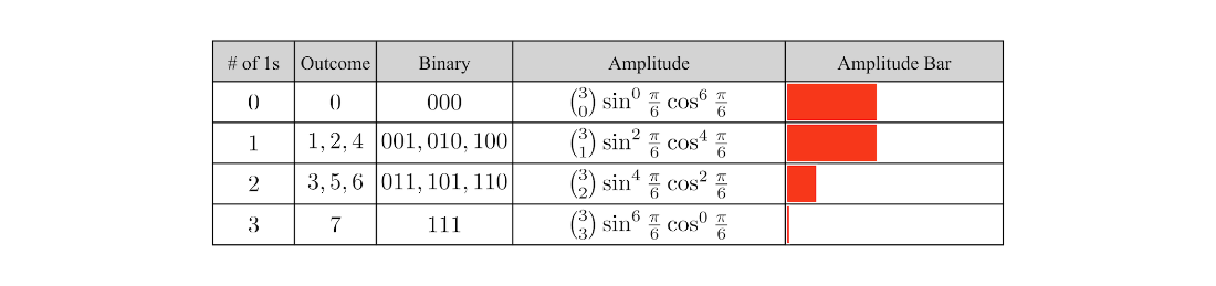
Table 4.15 The state table for the circuit that applies an \(R_Y(\theta)\)-rotation to \(n\) qubits. Here \(o(k)\) denotes the number of 1s in the binary expansion of \(k\).

Table 4.16 The general form of the three-qubit state prepared by applying \(R_Y(\theta)\) to every qubit.

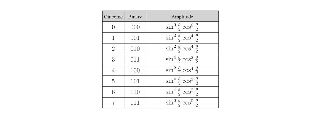
Table 4.17 The result of grouping outcomes with the same number of 1s.

Table 4.18 The uniform distribution prepared by applying \(R_Y(\pi/2)\) gates to every qubit.

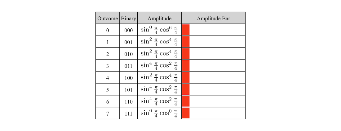
Table 4.19 The binomial distributions for \(p = \cos^2\frac{\pi}{2}\).

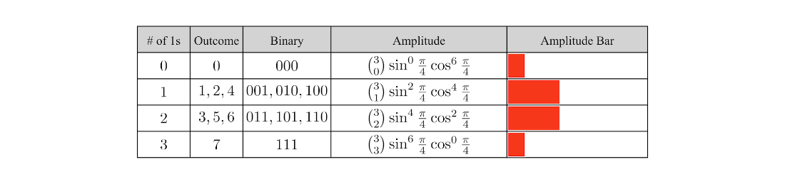
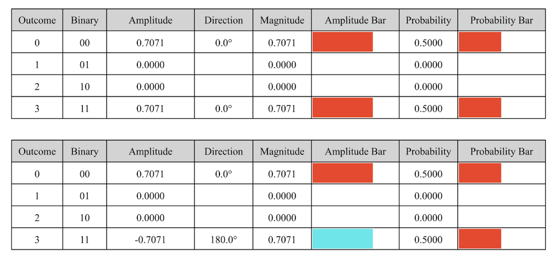
Table 4.20 The first Bell state table.

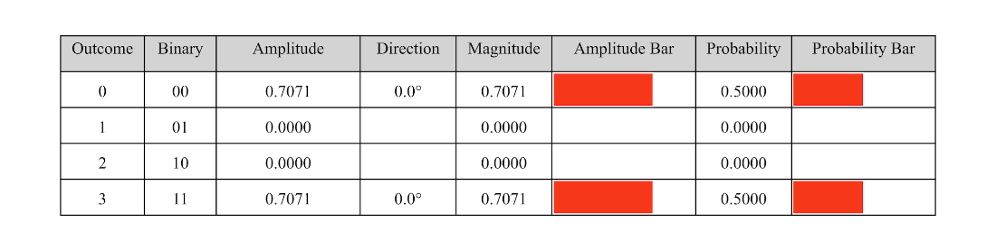
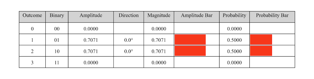
Table 4.21 The third Bell state table.

• A quantum system made up of \(n\) qubits can be represented by an array of \(2^n\) complex numbers, where the sum of squared magnitudes of the complex numbers is 1.
• State tables provide a visual way of understanding quantum states, connecting the mathematical and programmatic models.
• A quantum transformation applies a quantum gate to one qubit (the target qubit). It can also be controlled by using other qubits as control qubits.
• A quantum transformation recombines pairs of amplitudes determined by the target and control qubits according to the specific gate formula.
• Quantum circuits use quantum transformations to create useful states and probability distributions.
• Qubits can be organized into registers to make it easier to represent logical variables.
• We can write a simple Python simulator to simulate the basic principles of quantum computing.

FAQ