1 Understanding foundation models

Foundation models mark a shift from building narrow, data-specific models toward training a single, large model on vast and diverse datasets so it can be reused across many tasks. The chapter clarifies the difference between an algorithm (the recipe) and a model (the learned result on data) and defines key traits of foundation models: they are big (many parameters), trained on broad data, useful for multiple tasks, and adaptable via fine-tuning. In time series, this enables one model to forecast series with varied frequencies, trends, and seasonal patterns, and to tackle related tasks such as anomaly detection and classification, often working zero-shot and improving further with targeted fine-tuning.

The chapter introduces the Transformer, the backbone of most foundation models, from a time series perspective. Raw sequences are tokenized and passed through embeddings, then enriched with positional encoding so temporal order is preserved. The encoder’s multi-head self-attention learns dependencies (e.g., trends, seasonality) across the history, while the decoder uses masked attention to generate forecasts step by step without peeking into the future, guided by the encoder’s learned representation. A final projection maps deep representations back to forecast values, and predictions are fed back iteratively until the full horizon is produced. Many time series foundation models adopt this architecture wholesale, use decoder-only variants, or introduce task-specific adaptations.

Using foundation models offers practical benefits: quick, out-of-the-box pipelines; strong performance even with few local data points; lower expertise barriers; and reusability across datasets and tasks. The trade-offs include privacy considerations for hosted solutions, limited control over a model’s built-in capabilities, the possibility that a custom model may outperform in niche settings, and higher compute and storage requirements. The chapter sets expectations and boundaries for when these models excel, and previews hands-on work with several time series foundation models, applying zero-shot and fine-tuned forecasting to real datasets, exploring anomaly detection, extending language models to time series, and rigorously evaluating against traditional statistical baselines.

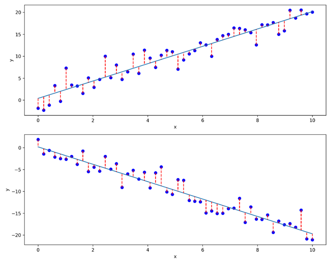
Result of performing linear regression on two different datasets. While the algorithm to build the linear model stays the same, the model is definitely very different depending on the dataset used.

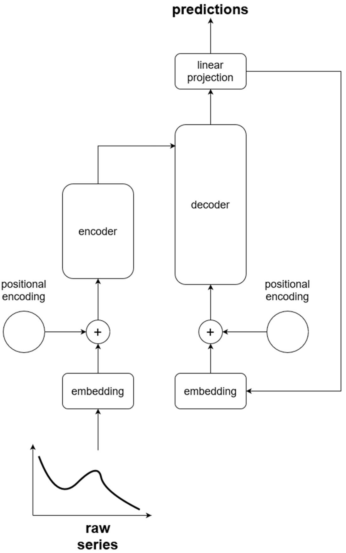
Simplified Transformer architecture from a perspective of time series. The raw series enters at the bottom left of the figure, flows through an embedding layer and positional encoding before going into the decoder. Then, the output comes from the decoder one value at a time until the entire horizon is predicted.

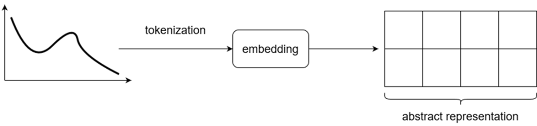
Visualizing the result of feeding a time series through an embedding layer. The input is first tokenized, and an embedding is learned. The result is the abstract representation of the input made by the model.

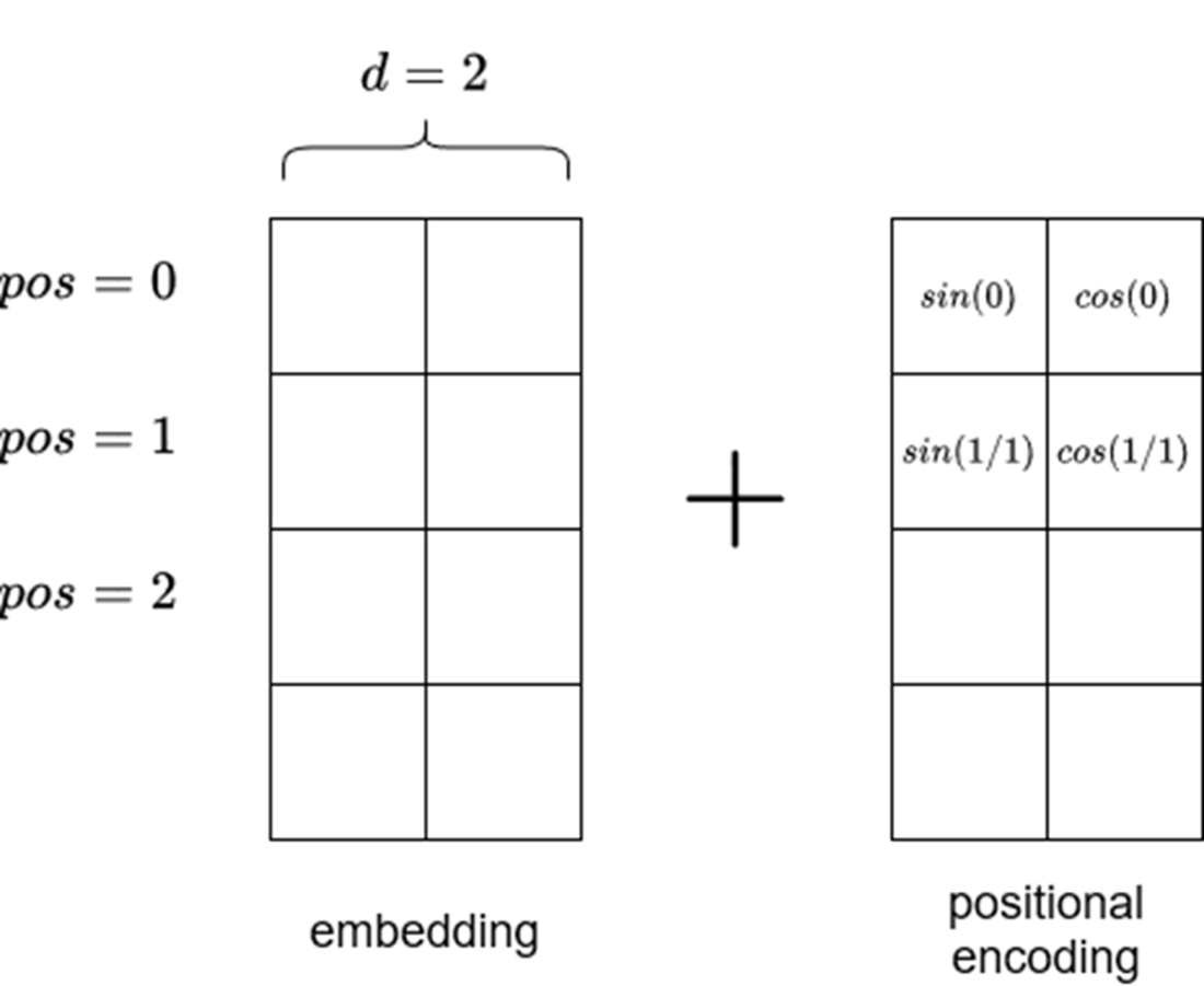
Visualizing positional encoding. Note that the positional encoding matrix must be of the same size as the embedding. Also note that sine is used in even positions, while cosine is used on odd positions. The length of the input sequence is vertical in this figure.

We can see that the encoder is actually made of many encoders which all share the same architecture. An encoder is made of a self-attention mechanism and a feed forward layer.

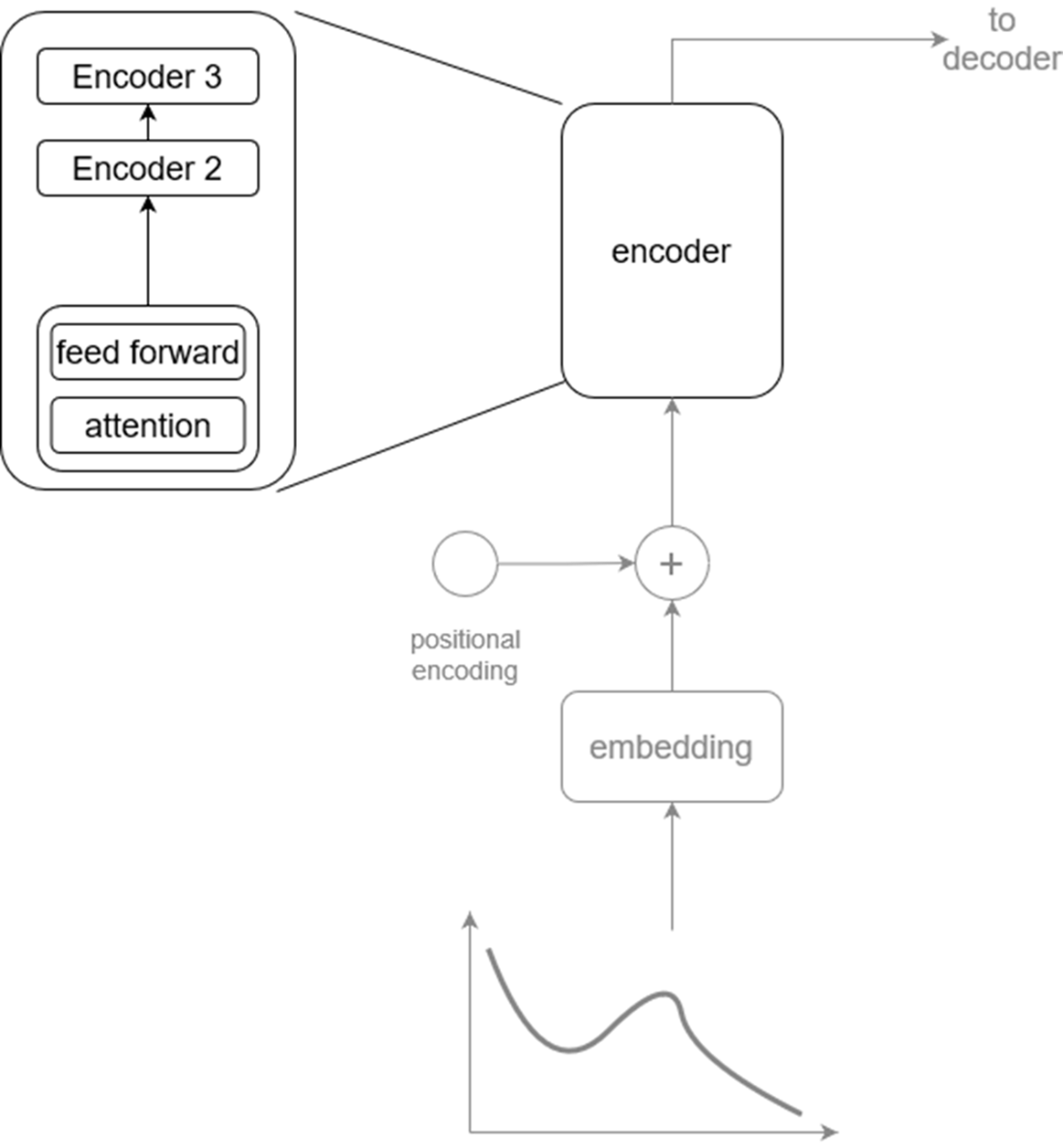
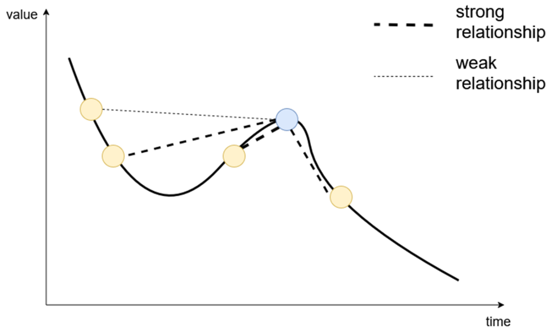
Visualizing the self-attention mechanism. This is where the model learns relationships between the current token (dark circle) and past tokens (light circles) in the same embedding. In this case, the model assigns more importance (depicted by thicker connecting lines) to closer data points than those farther away.

Visualizing the decoder. Like the encoder, the decoder is actually a stack of many decoders. Each is composed of a masked multi-headed attention layer, followed by a normalization layer, a multi-headed attention layer, another normalization layer, a feed forward layer, and a final normalization layer. The normalization layers are there to keep the model stable during training.

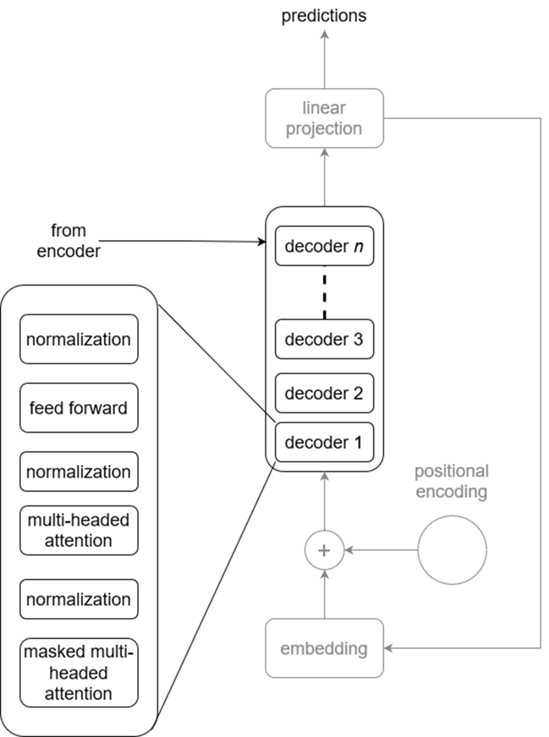
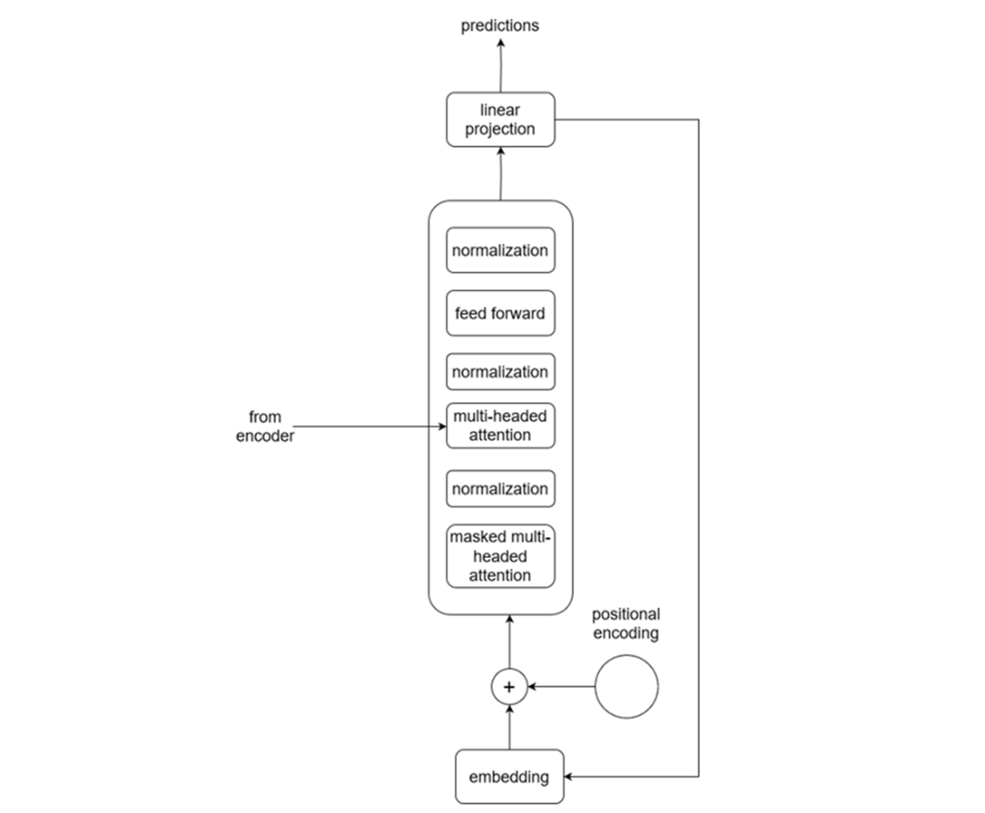
Visualizing the decoder in detail. We see that the output of the encoder is fed to the second attention layer inside the decoder. This is how the decoder can generate predictions using information learned by the encoder.

• A foundation model is a very large machine learning model trained on massive amounts of data that can be applied on a wide variety of tasks.
• Derivatives of the Transformer architecture are what powers most foundation models.
• Advantages of using foundation models include simpler forecasting pipelines, a lower entry barrier to forecasting, and the possibility to forecast even when few data points are available.
• Drawbacks of using foundation models include privacy concerns, and the fact that we do not control the model’s capabilities. Also, it might not be the best solution to our problem.
• Some forecasting foundation models were designed with time series in mind, while others repurpose available large language models for time series tasks.

FAQ