This chapter lays the foundation for building low‑latency applications by unifying core concepts, practical techniques, and mental models that are often scattered across folklore and blog posts. It introduces latency as a first-class performance concern, explains how to reason about it across the entire stack, and frames why it matters to product outcomes, real-time guarantees, and efficiency. The discussion previews key distinctions and trade-offs—especially against throughput and bandwidth—and sets expectations that optimizing latency frequently requires balancing physics, architecture, and workload behavior, including energy considerations.
Latency is defined as the time between a cause and its observed effect, a definition that scales from everyday interactions to complex distributed systems. Concrete examples—from the perceptible delay in smart or even some LED lighting to end‑to‑end web requests—illustrate how latency compounds across clients, networks, services, and rendering, and how variance directly shapes user experience. The chapter highlights that latency exists at every layer, down to packet handling from NIC queues through the kernel to userspace, and must be measured in units of time that span nanoseconds to milliseconds and beyond. Physical limits, such as the speed of light, bound what is achievable and make strategies like co‑location and careful system design essential when targets are tight.
Latency matters for three primary reasons: it drives user satisfaction and business outcomes, it underpins real‑time guarantees (hard vs. soft deadlines), and it often equates to efficiency in an era where free speedups from hardware have plateaued. The chapter distinguishes latency from bandwidth and throughput, emphasizing that while capacity can often be scaled, poor latency is stubborn—and sometimes must be traded against higher throughput, as with pipelining analogies. Finally, it surfaces the tension between latency and energy: techniques like busy polling can reduce response time yet raise power usage, though under steady, high‑frequency traffic they may also improve total energy efficiency. The overarching message is to optimize with clear goals, realistic constraints, and workload‑aware trade‑offs.
60 ms Length of a nanosecond. Source: https://americanhistory.si.edu/collections/search/object/nmah_692464
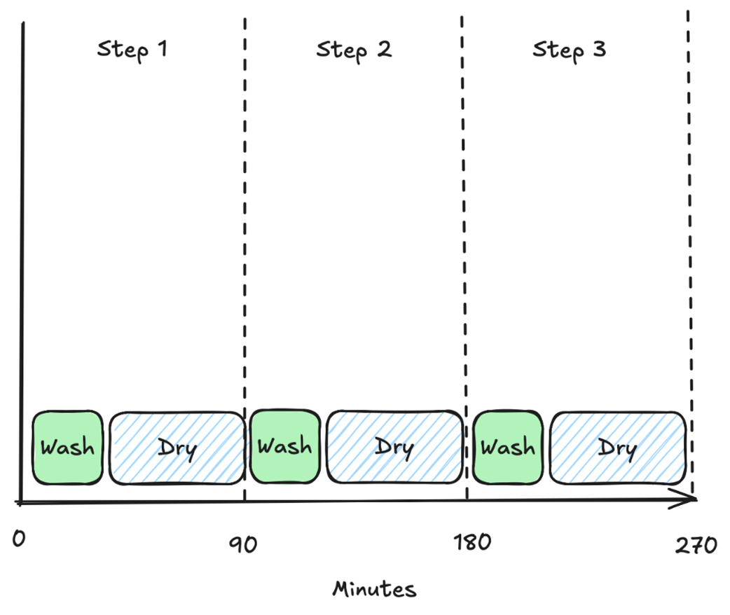
Processing without pipelining. We first perform step W (washing) fully and only then perform step D (drying). As the time to complete W is 30 minutes and the time to complete D is 60 minutes, each step takes 90 minutes in total. Therefore, we say that the latency to wash and dry clothes is 90 minutes and the throughput is 1/90 loads of laundry washed per minute.
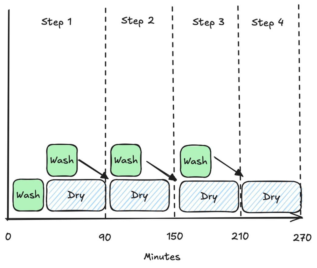
Processing with pipelining. We perform step W (washing) in full, but as soon as it completes, we start another step W. In parallel, we perform step D (drying) for the previous step W. If we ignore the initial step where there is no completed step W, the time to complete a load of laundry is 120 minutes because W and D run in parallel, but we’re bottlenecked by D, making latency worse than without pipelining. However, due to pipelining, we have now increased throughput to 1/60 loads of laundry per minute, which means that we can complete four loads of laundry in the same time as non-pipelined does three.
Summary
Latency is the time delay between a cause and its observed effect.
Latency is measured in units of time.
You need to understand the latency constants of your system when designing for low latency.
Latency matters because people expect a real-time experience.
When optimizing for latency, there are sometimes throughput and energy efficiency trade-offs.
FAQ
What is latency?Latency is the time delay between a cause and its observed effect. In systems terms, it’s the time between initiating an action (such as sending a request) and when its outcome becomes observable (like receiving a response). What you measure as “cause” and “effect” depends on context, so the latency span can differ across use cases.How is latency measured?Latency is measured in units of time. Typical scales range from nanoseconds for CPU caches and DRAM, to microseconds for SSD/NVMe access, and milliseconds for network round trips. As rough anchors: an L1 cache hit is ~1 ns, DRAM ~100 ns, NVMe ~10 μs, SSD ~100 μs, and a packet from New York to London ~60 ms.How does this book use the terms latency and response time?Some sources define response time as service time plus wait time and reserve “latency” for the waiting part. This book uses a more general definition: latency is the time delay between a cause and an effect. Practically, service time is the request processing latency, wait time covers network and queuing latency, and response time is the total request latency observed by the user.What are intuitive examples of latency in everyday systems?Turning on lights illustrates latency as the delay between pressing a switch (cause) and light emission (effect); smart bulbs add network hops and make this delay visible, and even some LEDs can take up to ~2 seconds. On the web, end-to-end latency spans DNS lookup, TCP/HTTP exchange, server processing, downstream service calls (like databases), and client-side rendering—these stages compound overall delay.Why does latency matter for user experience and business outcomes?Humans perceive actions under ~100 ms as instant; ~1 s feels fast but noticeable; beyond ~10 s feels slow without progress feedback. Empirically, higher latency reduces engagement and conversions; studies have reported measurable drops in purchases and interactions from even modest slowdowns. In competitive markets with low switching costs, optimizing latency is a clear UX and business advantage.What’s the difference between hard and soft real-time requirements?Hard real-time systems must meet strict deadlines; missing one is a system failure with potentially catastrophic consequences (e.g., pacemakers, safety-critical sensors). Soft real-time systems tolerate occasional deadline misses with degraded quality rather than failure (e.g., audio/video streaming). This book focuses on broadly applicable low-latency techniques, touching real-time methods where relevant.How do latency, throughput, and bandwidth differ?Latency is how long a single operation takes from start to observable finish. Bandwidth is the maximum capacity of a channel (how much data could be moved per unit time). Throughput is the realized rate of successful work done (how much data or how many requests actually flow). Bandwidth sets an upper bound for throughput, but throughput and latency can vary independently, and the book emphasizes throughput over bandwidth when discussing data rates.Can improving throughput hurt latency? (The laundry/pipelining trade-off)Yes. In a serial “wash then dry” flow, latency is 30 + 60 = 90 minutes per load, with throughput of 1/90 loads per minute (~0.6 loads/hour). Pipelining overlapping wash and dry increases throughput to 1/60 loads per minute (1 load/hour) but raises per-load latency to ~120 minutes, illustrating a latency–throughput trade-off.What fundamental limits constrain latency?The speed of light sets a hard lower bound on how fast information can travel; practical media like fiber slow it further. These physical constraints mean some latencies cannot be optimized away and motivate techniques like co-location to reduce distance and hops.How does optimizing for latency interact with energy efficiency?Lower latency can conflict with energy goals. Techniques like busy polling reduce scheduling delays but consume constant power; sleep–wake strategies save energy but add wake-up latency. Depending on traffic patterns, busy polling may even be more energy-efficient at high request rates, while sporadic workloads favor sleeping—choose based on your latency targets and energy budget.
pro $24.99 per month
access to all Manning books, MEAPs, liveVideos, liveProjects, and audiobooks!