1 Introduction to Bayesian statistics: Representing our knowledge and uncertainty with probabilities
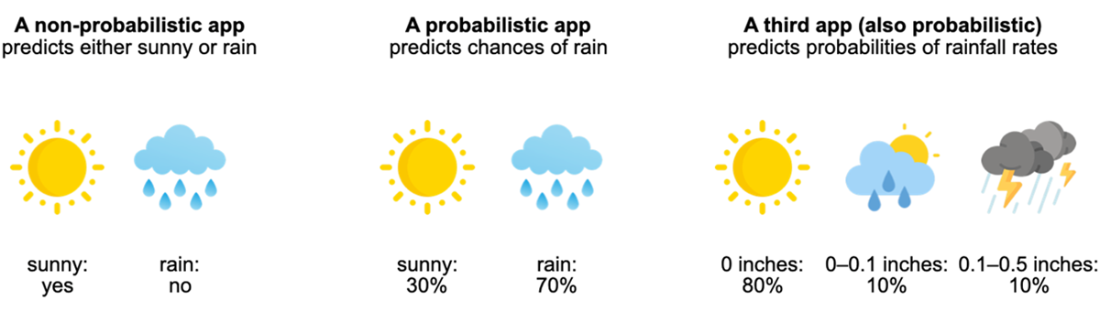
Bayesian statistics is introduced as a practical language for reasoning and decision-making under uncertainty. Instead of giving single, brittle answers, it represents what we know—and how sure we are—using random variables and probability distributions, then updates those beliefs as new evidence arrives. A weather-forecasting example motivates why probabilities matter: a simple yes/no prediction ignores inevitable error and users’ differing risk tolerances, while probabilistic forecasts enable better choices and inspire more trust. The chapter illustrates how different random variables (binary, categorical, continuous) provide varying levels of granularity, and how summaries like expected value help turn beliefs into actionable insights.
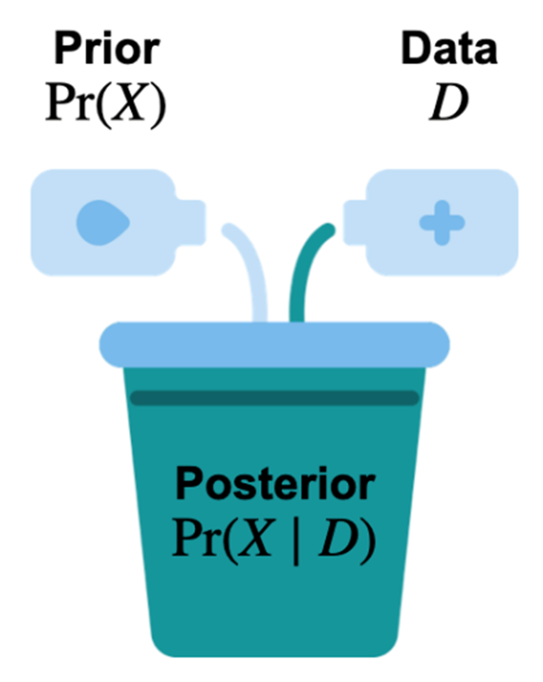
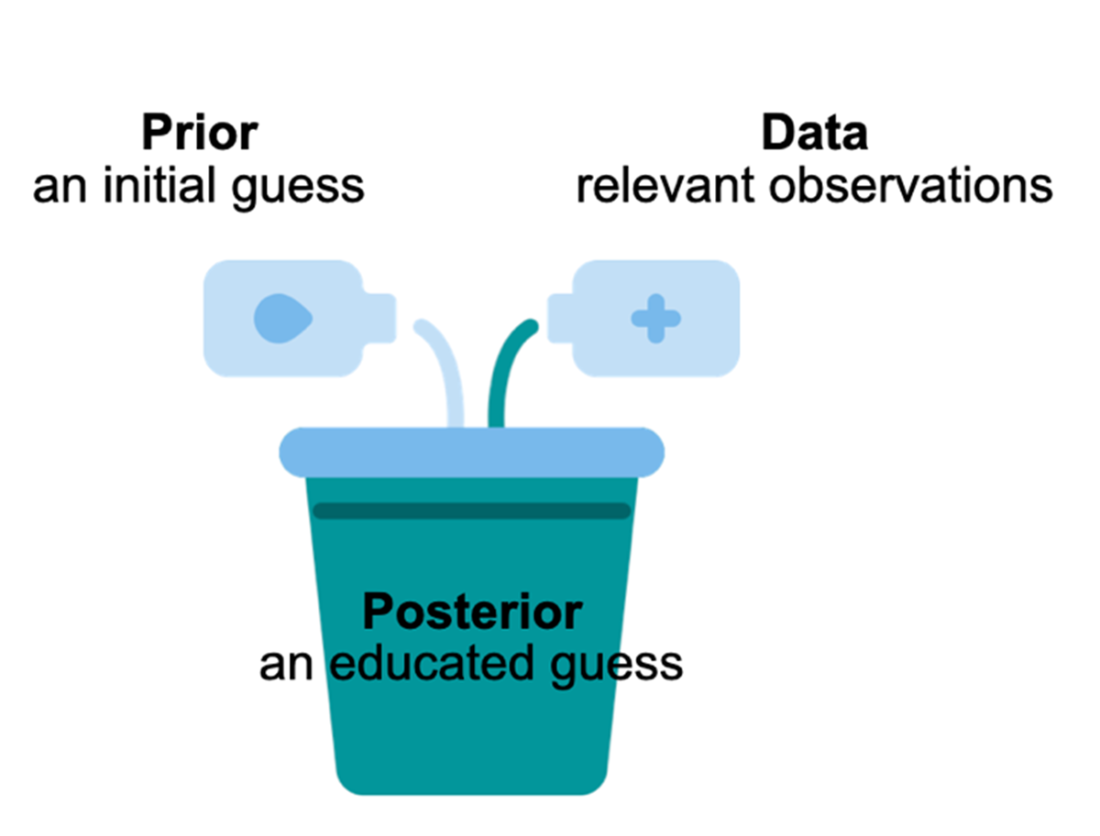
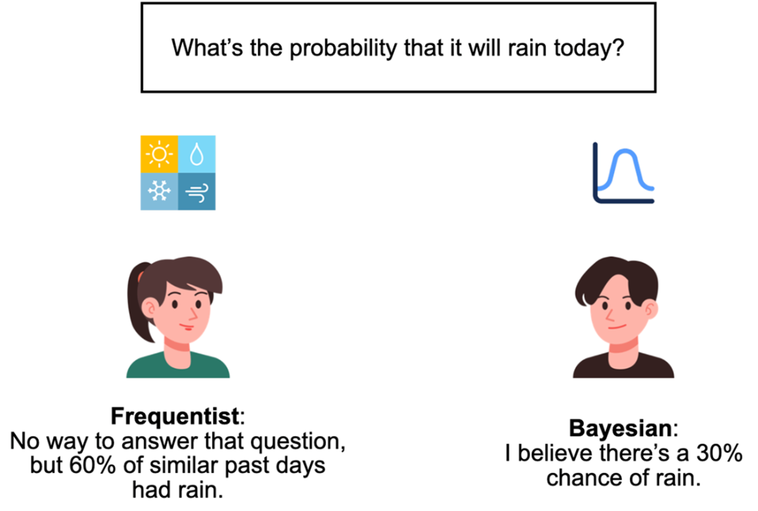
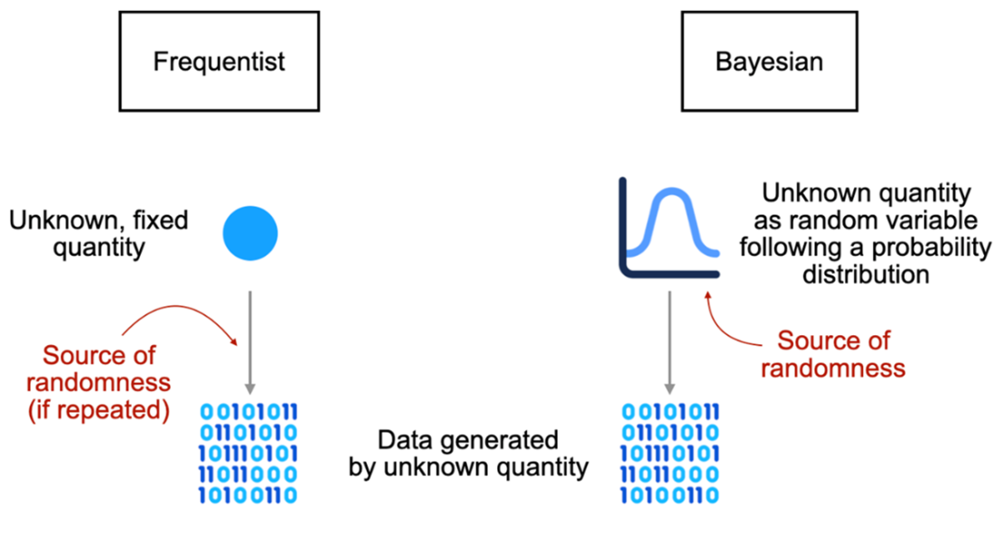
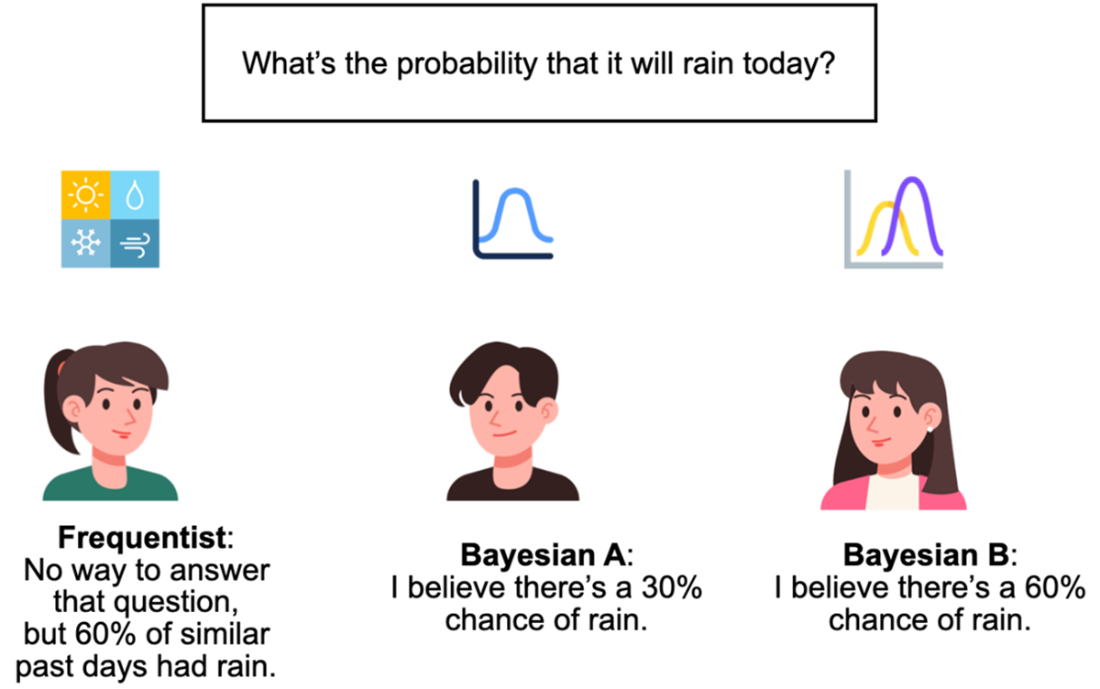
The Bayesian workflow centers on three components: a prior that encodes initial beliefs, data as observed evidence, and a posterior that combines the two to yield updated beliefs via conditional probabilities. This belief-updating mirrors everyday reasoning (e.g., revising rain odds after seeing dark clouds). The chapter contrasts this with frequentist statistics, which treats probability as long-run frequency from repeated trials and typically regards parameters as fixed. Frequentist methods are often computationally lighter and need less diagnostic work, while Bayesian methods are flexible, transparent about assumptions, and can leverage prior knowledge—especially valuable with limited data or high-stakes decisions. Although Bayesian inference is sometimes called “subjective,” the chapter frames that subjectivity as a strength that, together with sufficient data, often converges to robust conclusions.
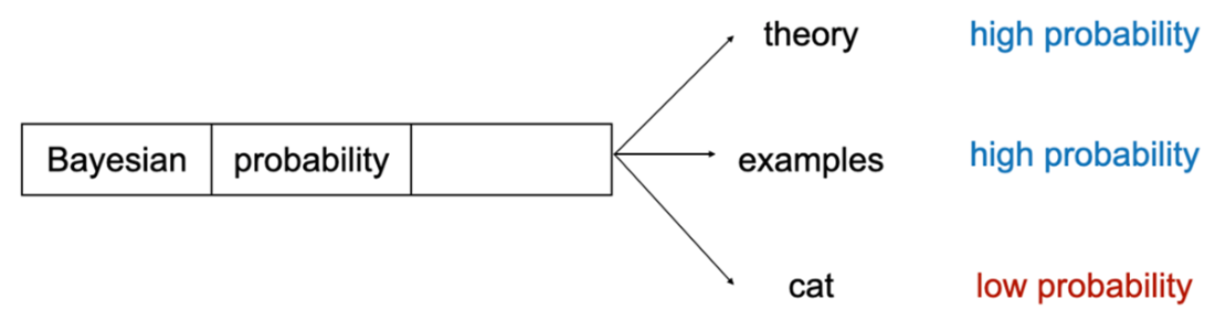
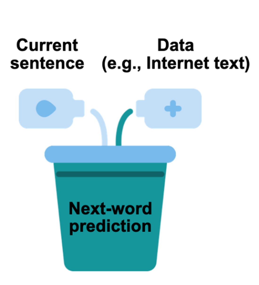
As a modern showcase, the chapter connects Bayesian thinking to large language models. Next-word prediction is inherently probabilistic: models score many plausible continuations conditioned on context and training data. While LLMs are not fully Bayesian—computing exhaustive posteriors over all possible words is intractable—they approximate by focusing on the most likely candidates, then sample multiple outputs to support user feedback and iterative refinement. This probabilistic machinery mitigates overconfident errors, aligns with real-world ambiguity, and underscores why Bayesian ideas permeate today’s AI systems. The chapter closes by positioning the book as an intuitive, visually guided path to building, interpreting, and applying Bayesian models to real-world problems.
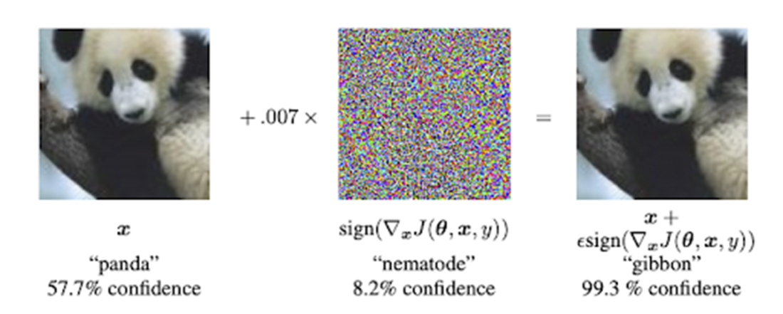
An illustration of machine learning models without probabilistic reasoning capabilities being susceptible to noise and overconfidently making the wrong predictions.
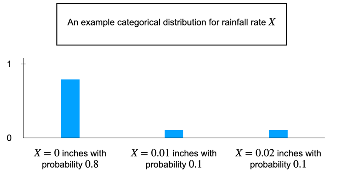
An example categorical distribution for rainfall rate.
Summary
We need probability to model phenomena in the real world whose outcomes we haven’t observed.
With Bayesian probability, we use probability to represent our personal belief about an unknown quantity, which we model using a random variable.
From a Bayesian belief about a quantity of interest, we can compute quantities that represent our knowledge and uncertainty about that quantity of interest.
There are three main components to a Bayesian model: the prior distribution, the data, and the posterior distribution. The last component is the result of combining the first two and what we want out of a Bayesian model.
Bayesian probability is useful when we want to incorporate prior knowledge into a model, when data is limited, and for decision-making under uncertainty.
A different interpretation of probability, frequentism, views probability as the frequency of an event under infinite repeats, which limits the application of probability in various scenarios.
Large language models, which power popular chat artificial intelligence models, apply Bayesian probability to predict the next word in a sentence.
FAQ
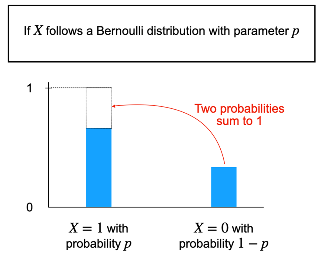
What is Bayesian statistics and why should I use it?Bayesian statistics is a framework for reasoning under uncertainty. It represents what you currently believe about an unknown quantity with a probability distribution, then updates that belief when new evidence arrives. This lets you make predictions and decisions that reflect both your data and your uncertainty—useful in everyday choices (like bringing an umbrella) and in domains like medical diagnostics, recommendation systems, and AI.Why are probabilistic predictions better than simple yes/no answers?Yes/no outputs hide uncertainty. Probabilistic predictions expose how confident we should be, enabling decisions that match different risk tolerances. A weather app that says “30% chance of rain” lets a short-distance runner skip an umbrella while someone outdoors all day might bring one. More granular probabilities (for specific rainfall amounts) carry even more useful information.What is a random variable, and what types are common in practice?A random variable represents an unknown outcome in a probabilistic experiment. Common types include: binary (two outcomes, like rain vs. no rain), categorical (one of several discrete categories, such as binned rainfall amounts), and continuous (any value in a range, like exact rainfall rate). Choosing between them balances granularity and practicality.What is a probability distribution and what do its parameters mean?A probability distribution assigns likelihoods to the possible values of a random variable subject to the axioms that probabilities are nonnegative and sum to 1. Distributions are governed by parameters that control their behavior. For example, a Bernoulli distribution has parameter p: the probability of “success” (e.g., rain = 1) is p, and “failure” (no rain = 0) is 1 − p.How do priors, data, and posteriors work in a Bayesian model?The prior encodes your initial belief about an unknown quantity before seeing data. The data are the evidence you observe. The posterior is your updated belief after combining prior and data, expressed as a conditional probability (often written as Pr(X | D)). For example, you might start with a low prior for rain, observe dark clouds (data), and update to a higher posterior probability of rain.How does Bayesian probability differ from frequentist probability?Bayesian probability quantifies a degree of belief about unknowns and updates it with evidence. Frequentist probability defines probability as a long-run frequency across repeated trials. A Bayesian can assign a probability to “rain today” based on current evidence; a frequentist reframes the question in terms of frequencies over many similar days. With abundant data, both approaches can yield similar answers, though via different interpretations.When should I use Bayesian methods versus frequentist methods?Use Bayesian methods when you want to incorporate domain knowledge as priors, when data are limited, or when you need customized decision analysis. Use frequentist methods when data are abundant, when prior knowledge isn’t needed, or when established tools like classical hypothesis tests and A/B tests suit the objective.What is the expected value and what does it tell me?The expected value is the probability-weighted average of a random variable’s possible values. It summarizes the variable’s central tendency but is not necessarily the value you’ll observe. Example: if rainfall is 0 with probability 0.8, 0.01 with 0.1, and 0.02 with 0.1, the expected rainfall is 0×0.8 + 0.01×0.1 + 0.02×0.1 = 0.003 inches per hour.Why do machine learning models benefit from probabilistic reasoning?Deterministic models can be overconfident and brittle to noise (e.g., small input perturbations causing confidently wrong predictions). Probabilistic reasoning helps quantify uncertainty, reducing overconfidence—crucial in high-stakes settings like healthcare. Note that classifier scores normalized by softmax are convenient but aren’t guaranteed to be well-calibrated probabilities.How do Bayesian ideas show up in large language models (LLMs), and why aren’t LLMs fully Bayesian?LLMs are next-word predictors that model conditional probabilities of words given context and training data. This is “Bayesian in spirit” because it reasons with uncertainty over many plausible next words. Fully computing a posterior over the entire vocabulary is too expensive, so LLMs approximate by focusing on the most likely candidates and sampling. Keeping multiple likely candidates also enables user feedback to refine the model after training.
pro $24.99 per month
access to all Manning books, MEAPs, liveVideos, liveProjects, and audiobooks!
 Grokking Bayes ebook for free