9 Quantum phase estimation
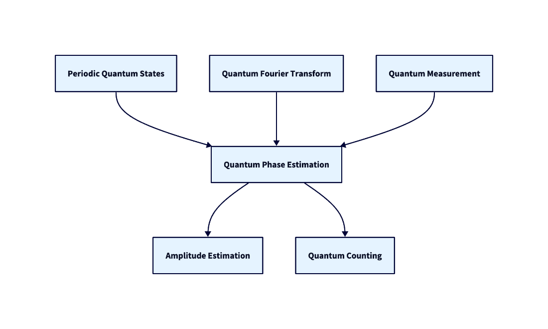
This chapter builds on the quantum Fourier transform to introduce quantum phase estimation (QPE), a core primitive often called the “Swiss army knife” of quantum computing and a key component of algorithms like Shor’s. The central goal is to estimate an unknown circuit phase (rotation angle) by turning phase into measurable frequency information. The narrative progresses from encoding values as periodic quantum states and reading them out via inverse QFT, through the concepts of eigenstates and eigenvalues that make QPE possible, and culminates with amplitude estimation—an algorithm that leverages QPE ideas to estimate probabilities and counts (quantum counting) far more efficiently than naive sampling.
The chapter first shows how to encode a value as the frequency of a phased discrete sinc state and recover it statistically by repeated measurements. Using more qubits refines resolution (more “ticks” on the ruler), and when the encoded value is non-integer the probability mass concentrates on the nearest integers. Beyond taking the most frequent outcome, accuracy improves by interpolating between the two closest outcomes, notably with a simple and effective estimator using magnitudes: sqrt(pa)/(sqrt(pa)+sqrt(pb)). With the relationship theta/(2π) = v/2^n, QPE is then presented step by step: prepare an eigenstate of a unitary U on a target register, put an estimation register into superposition, apply controlled powers of U (growing exponentially), optionally unprepare the eigenstate, and apply the IQFT to the estimation register to extract an estimate of the eigenphase. Two circuit realizations are discussed—one that uses the standard IQFT with swaps and an alternative that avoids swaps by reversing qubit order—both yielding the same final estimation state.
Amplitude estimation adapts this framework by using the Grover iterate as the unitary whose eigenphase encodes the desired amplitude. The circuit mirrors QPE: prepare the target state (operator A), put the estimation register into superposition, apply controlled powers of the Grover iterate, and finish with an IQFT. From the most frequent estimation outcome v, one estimates the probability of “good” outcomes as sin²(π v / 2^n) and, when outcomes are equiprobable, the count as approximately 2^m sin²(π v / 2^n). Compared with classical sampling, amplitude estimation achieves the same precision with exponentially fewer measurements (at the cost of deeper circuits and more qubits), enabling tasks like quantum counting (estimating how many items satisfy an oracle) and probability estimation for arbitrary state preparations.
A dependency diagram of concepts covered in this chapter.
The circuit for encoding a frequency value \(v\) in a quantum state with \(n\) qubits, where \(\theta = v \frac{2 \pi}{2^n}\).

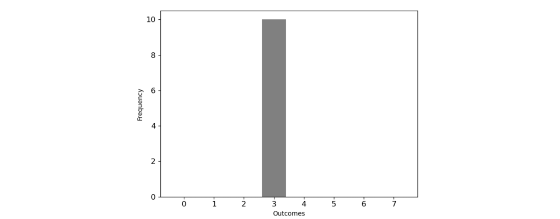
Measurement outcome frequencies from 10 shots of a phased discrete sinc state with \(n = 3\) qubits and the encoded frequency value \(v = 3\).
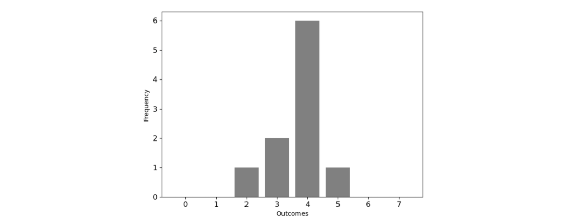
Measurement outcome frequencies from 10 shots of a phased discrete sinc state with \(n = 3\) qubits and the encoded frequency value \(v = 3.8\).
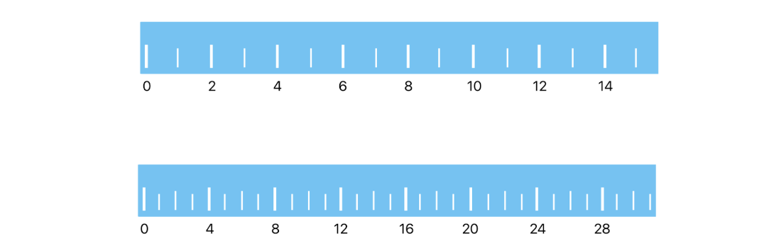
Using \(n = 3\) qubits is like using a ruler with eight ticks.

Using one more qubit (\(n = 4\)) doubles the number of ticks on the ruler. Using \(n = 5\) qubits doubles the number of ticks again.
The measurement outcome probabilities for a phased discrete sinc state with \(n = 3\) qubits and the encoded frequency value \(v = 4.76\).

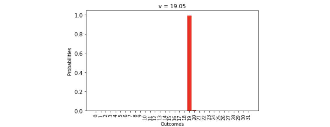
The measurement outcome probabilities for a phased discrete sinc state with \(n = 5\) qubits and the encoded frequency value \(v = 19.05\).
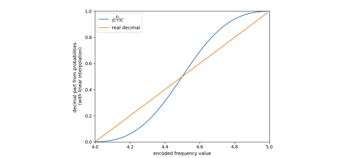
Real decimal value versus the approximation from the ratio of frequencies of the two closest integers.
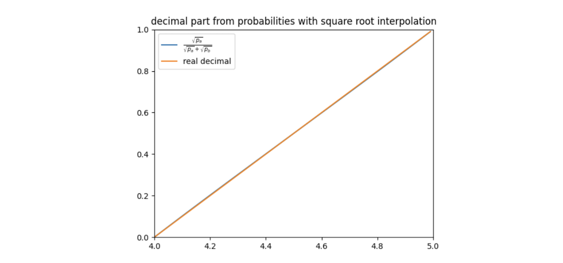
Real decimal value versus the approximation from the ratio of the approximate magnitudes of the two closest integers.
The effect of a quantum circuit \(U\) when applied to one of its eigenstates.

A single qubit circuit \(U = R_Y(2 \theta)\).

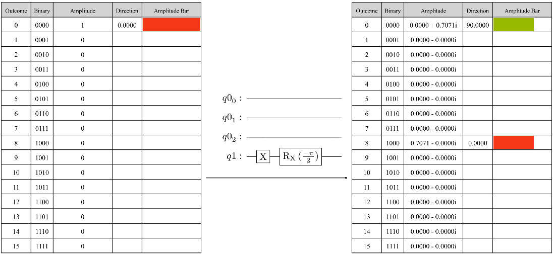
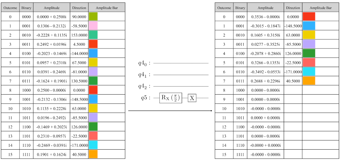
A single-qubit state in its' default state and after applying the circuit \(R_X \left(\frac{-\pi}{2} \right) X\).

The state tables before and after applying the circuit \(R_Y \left( \frac{\pi}{3} \right)\).
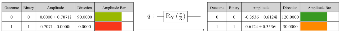
The color wheel visualization of the amplitudes of a single-qubit state before and after the circuit \(R_Y \left( \frac{\pi}{3} \right)\) is applied.

The state table after applying the circuit \(R_Y \left( \frac{\pi}{3} \right)\) twice.
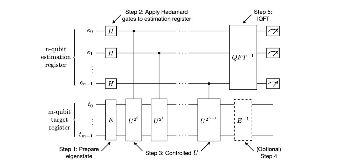
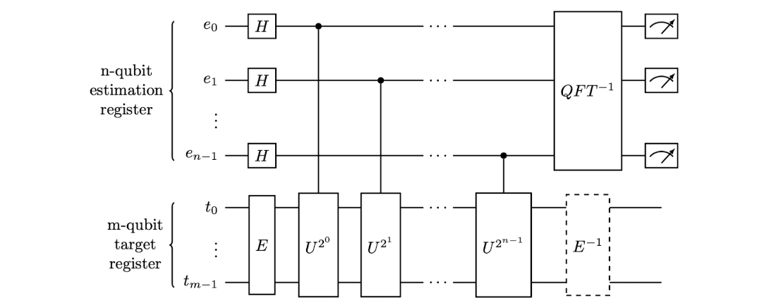
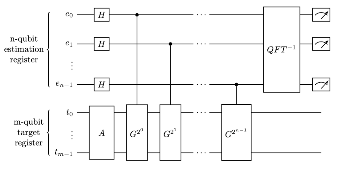
The phase estimation algorithm where \(U\) is an \(m\)-qubit circuit and \(E\) prepares an eigenstate of the circuit.
The initial state table and the state table after applying the circuit \(R_X \left(\frac{-\pi}{2} \right) X\) to the target register.
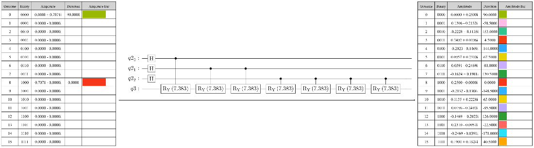
The state table where an eigenstate is prepared in the target register, the circuit that applies Hadamard gates to each qubit in the estimation register, followed by controlled applications of the circuit \(R_Y (2 \theta )\).
The state table of geometric sequence states in superposition, the inverse of the circuit that prepared the eigenstate, and the resulting geometric sequence state in the estimation register.
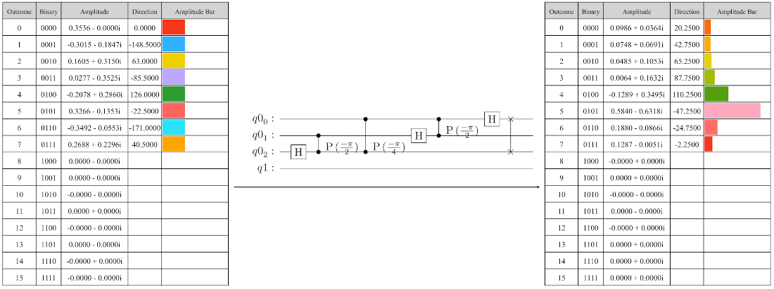
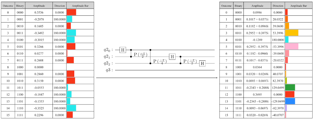
The state table of geometric sequence states in superposition, the IQFT applied to the estimation register, and the state table of the superposition of phased discrete sinc states.
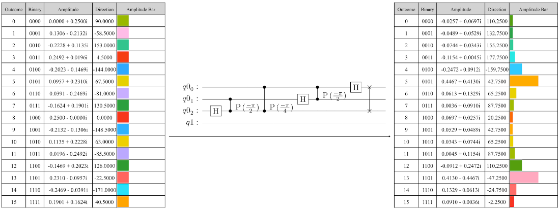
The state table of geometric state in the estimation register, the IQFT applied to the estimation register, and the state table of the resulting phased discrete sinc state.
The phase estimation algorithm where \(U\) is an \(m\)-qubit circuit and \(E\) prepares an eigenstate of the circuit.
The state table where an eigenstate is prepared in the target register and the state table of the geometric sequence state with amplitudes in reversed order (previous amplitudes [0, 1, 2, 3, 4, 5, 6, 7] map to amplitudes [0, 4, 2, 6, 1, 5, 3]).
The state table of the geometric sequence state with qubits in reverse order, the circuit for applying the IQFT to the estimation register in reverse order and without qubit swaps, and the resulting state table for the phased discrete sinc state.
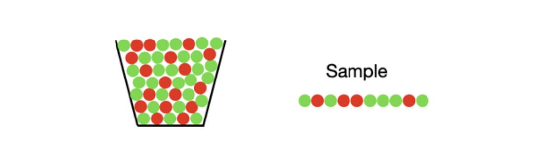
Samples taken from a large bin of marbles.
Circuit diagram of the amplitude estimation algorithm.
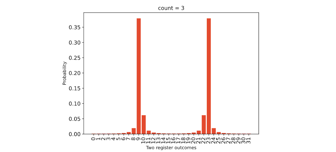
Measurement outcome probabilities of the estimation register.
Measurement probabilities of the second half of the estimation register outcomes.
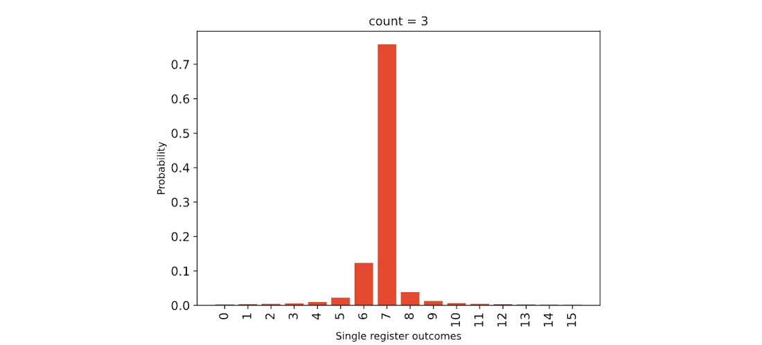
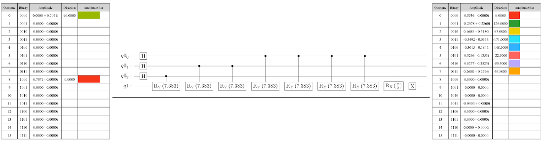
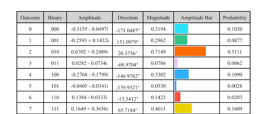
Table 9.1 A three-qubit state prepared with a randomly generated circuit.
Summary
- If we have measurement results from a phased discrete sinc state with \(n\) qubits and an unknown encoded frequency value \(v\), we can get an estimate for the true value of \(v\), and the corresponding angle parameter \(\theta = v \frac{2 \pi}{2^n}\). In this chapter, we learned two methods for getting an estimate:
- The first method is to approximate the encoded frequency value \(v\) by the most frequent integer outcome. We can approximate the angle parameter \(\theta\) using \(\theta = v \frac{2 \pi}{2^n}\).
- The second method used the ratio of the approximate magnitudes of the two most frequent consecutive integer outcomes. We denote the smaller of the two most frequent outcomes by \(b\) (for below) and the larger by \(a\) (for above). We denote the proportion of outcomes \(a\) and \(b\) by \(p_a\) and \(p_b\), respectively. We estimate the integer part of the encoded frequency value to be \(a\), and the decimal part to be
- A quantum state vector is called an eigenvector (or eigenstate) of a circuit transformation \(U\), if all its amplitudes are multiplied by a corresponding eigenvalue (a complex number of length 1) as a result of the circuit application.
- Given an \(m\)-qubit circuit \(U\) (where \(m > 1\)), we can implement the phase estimation circuit to create a phased discrete sinc state in the estimation register. We can use the state created to get an estimate for the phase of eigenvalue corresponding to the eigenstate using the methods covered in this chapter, or more advanced methods (such as MLE).
- The amplitude estimation algorithm estimation can be used to estimate the number of good outcomes, called quantum counting, or estimate the probability of good outcomes.
FAQ
What is quantum phase estimation (QPE) and why is it important?
QPE estimates the unknown phase (rotation angle) associated with an eigenvalue of a unitary circuit U by converting that phase into a measurable frequency on an estimation register. It’s a core building block for many algorithms, including Shor’s factoring algorithm, amplitude estimation, and various simulation and optimization routines.How do you encode and estimate the frequency of a periodic quantum state?
Prepare a geometric sequence state on n qubits (apply Hadamards, then phase rotations that encode the phase differences), apply the inverse QFT (IQFT) to convert phase to magnitude, then measure. If the encoded value v is an integer, you obtain that outcome with probability 1. If v is not an integer, outcomes concentrate around the nearest integers; with one measurement the closest integer appears with probability at least 4/π² (~40%), and one of the two nearest integers with probability at least 8/π² (~81%).What is the relationship between the frequency v, the angle θ, and the number of qubits n?
The parameters satisfy θ/(2π) = v/2ⁿ. For a fixed θ, increasing n scales the encoded frequency: vₙ = 2ⁿ⁻ᵐ vₘ (for n > m). If v is outside [0, 2ⁿ), the estimate effectively returns v mod 2ⁿ, because frequencies differing by 2ⁿ correspond to the same rotation (angles wrap modulo 2π).Why do more qubits improve phase (angle) estimation precision?
Measurement outcomes act like tick marks on a ruler. With n qubits there are 2ⁿ ticks. More qubits double the number of ticks each time, shrinking the spacing and allowing finer resolution of the true value between ticks.Can we improve non-integer estimates beyond “closest tick” and how?
Yes. Interpolate between the two most likely neighboring outcomes:- Using probabilities p_a (above) and p_b (below): decimal ≈ p_a / (p_a + p_b).
- Using magnitudes (square roots): decimal ≈ √p_a / (√p_a + √p_b), which is notably more accurate and approaches an exact formula as 2ⁿ grows.
- Other methods like maximum likelihood estimation (MLE) can also help, but the two-outcome magnitude ratio is simple and effective for phased discrete sinc states.
What are eigenstates and eigenvalues in the context of QPE?
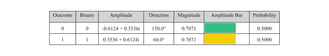
An eigenstate |ψ⟩ of a unitary U is a state that U maps to λ|ψ⟩, where λ has unit magnitude and equals cis(θ) = e^{iθ}. All amplitudes are rotated by the same angle θ. Example: for U = RY(2θ), the state [i/√2, 1/√2] is an eigenstate with eigenvalue cis(θ). Repeated applications of U rotate the state by θ each time without changing magnitudes.How does the quantum phase estimation circuit work, step by step?
- Create two registers: an n-qubit estimation register and an m-qubit target register.
- Prepare an eigenstate of U on the target register (eigenvalue phase θ).
- Apply Hadamards to all estimation qubits.
- For each estimation qubit k, apply controlled-U^{2^k} to the target.
- (Optional) Uncompute the eigenstate on the target to leave a single geometric sequence on the estimation register.
- Apply IQFT to the estimation register.
- Measure and convert the most frequent outcome (or an interpolated value) v to θ via θ ≈ 2π v / 2ⁿ.
What’s the alternative QPE implementation without qubit swaps and why use it?
The alternative applies the controlled powers in reverse order and then runs the IQFT in reversed qubit order without final swaps. This reorders the intermediate amplitudes (e.g., outcome labels are bit-reversed), but yields the same final phased discrete sinc state. It saves swap operations and can be more efficient on hardware with limited connectivity.What is amplitude estimation and how is it related to QPE?
Amplitude estimation uses QPE on the Grover iterate G = A M₀ A⁻¹ O (built from a state-preparation circuit A and an oracle O). G acts as a rotation by 2θ where sin²θ equals the success probability. Running QPE on G yields an estimate v on n qubits, from which we estimate:- Success probability ≈ sin²(π v / 2ⁿ).
- If all outcomes are equally likely, the number of “good” outcomes ≈ 2ᵐ sin²(π v / 2ⁿ), enabling quantum counting.
How many measurements (shots) and qubits do I need for accurate estimates?
- Shots: Statistical error decreases with more measurements. Hoeffding’s inequality bounds the deviation probability by 2 exp(−2 ε² M), where M is the number of samples (shots).
- Estimation qubits: More qubits improve resolution (spacing 1/2ⁿ). Use interpolation to “read between ticks” if you can’t add qubits.
- Note: Simulated measurement outcomes vary between runs due to sampling randomness; more shots stabilize frequency estimates.
 Building Quantum Software with Python ebook for free