Algorithms and data structures are presented as practical tradeoffs: every choice affects speed, memory use, and scalability. The chapter begins by contrasting arrays and linked lists, showing that textbook complexity is only part of the story. Arrays provide fast indexed access and strong cache locality because their elements are contiguous in memory, while linked lists can make insertions and deletions cheap when the insertion point is already known. In practice, however, linked lists often suffer from pointer overhead, poorer cache behavior, and less predictable memory access, so performance-sensitive decisions should be benchmarked rather than based only on Big-O notation.
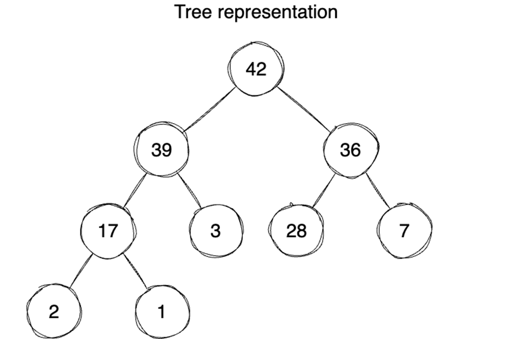
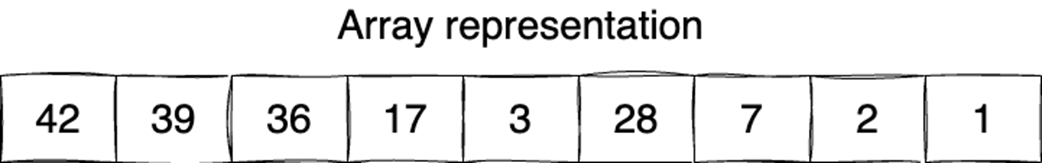
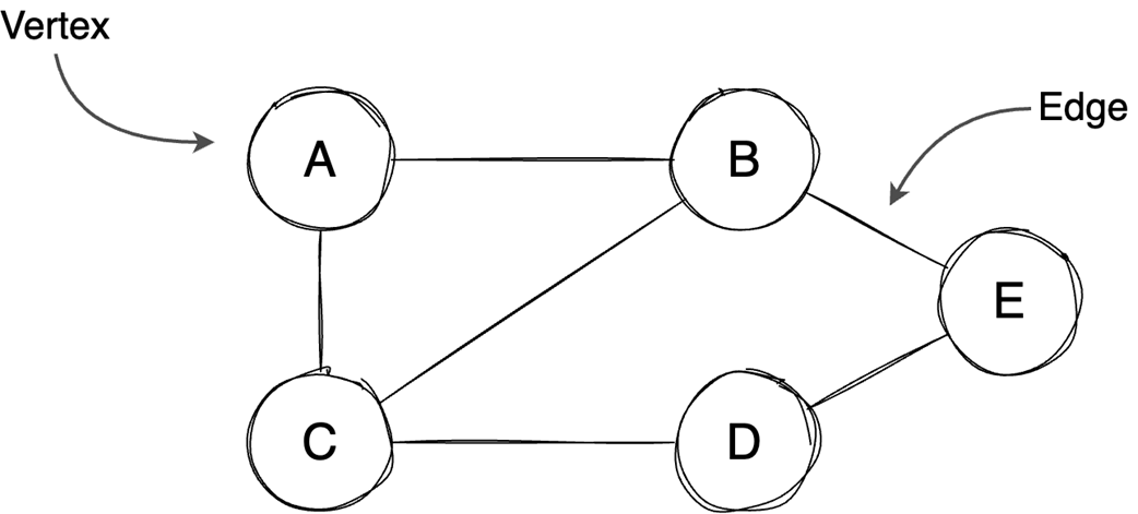
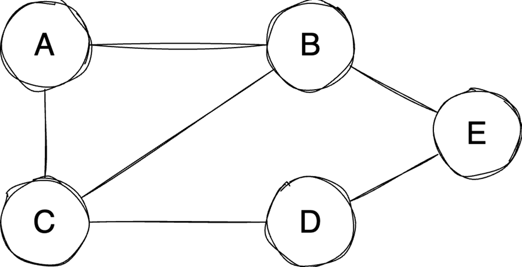
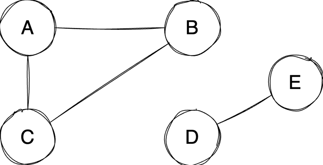
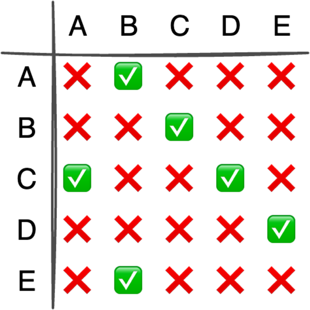
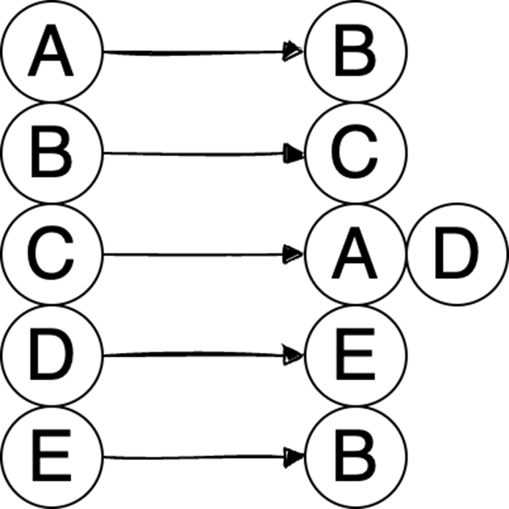
The chapter then moves from general containers to specialized structures and relationship-based models. Binary heaps are introduced as an efficient way to retrieve either the minimum or maximum element quickly, making them well suited for priority queues and algorithms such as Dijkstra’s algorithm or heapsort. Heaps are typically stored in arrays, support constant-time access to the top element, and use heapify operations to keep insertion and extraction logarithmic. Graphs extend the discussion to data defined by relationships between vertices and edges, with important properties such as direction, cycles, weights, and connectivity. The text compares adjacency matrices, which give constant-time edge lookup but can waste space, with adjacency lists, which are more space-efficient for sparse graphs but slower for edge lookup.
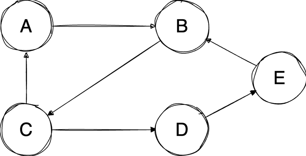
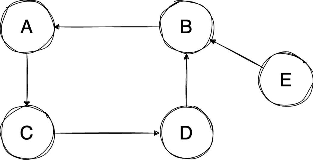
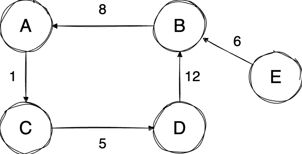
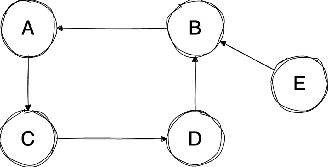
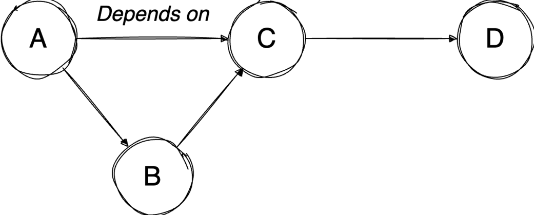
The final part focuses on graph algorithms that exploit specific graph properties. Topological sorting works on directed acyclic graphs to produce a valid execution order for dependent tasks, using in-degree counts and a queue of vertices with no remaining prerequisites; it is useful in build systems, package managers, and deadlock detection. The Ford-Fulkerson algorithm addresses maximum flow problems by repeatedly finding augmenting paths, pushing the bottleneck flow through them, and updating residual capacities, including backward edges that allow previous flow choices to be corrected. Its complexity depends on how augmenting paths are chosen: a DFS-based version depends on the maximum flow value, while the BFS-based Edmonds-Karp variant depends only on graph structure. Overall, the chapter emphasizes that the key skill is recognizing which data-organization or algorithmic tradeoff a problem demands.
Summary
Arrays and linked lists represent a trade-off between access speed and flexibility: Arrays provide instant index-based access and better cache locality, whereas linked lists allow for dynamic growth and efficient insertions at the cost of memory overhead and cache misses.
Binary heaps are the ideal structure for priority queues: By maintaining a specific tree property, they offer O(1) access to the minimum or maximum element and O(log n) efficiency for updates.
Graph representation depends on density: Adjacency matrices offer O(1) edge lookups but consume O(V²) space, making them suitable for dense graphs, while adjacency lists are more space-efficient for sparse graphs.
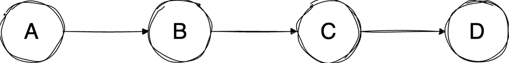
Topological sort resolves dependencies: This algorithm linearly orders vertices in a Directed Acyclic Graph (DAG) ensuring that for every dependency A to B, A comes before B in the ordering.
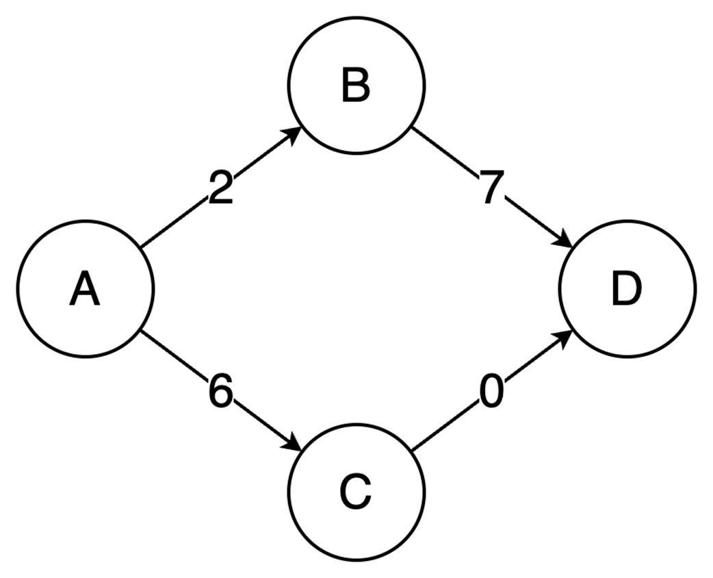
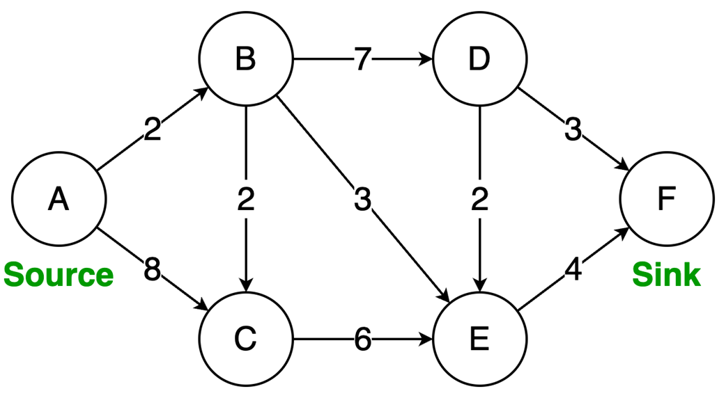
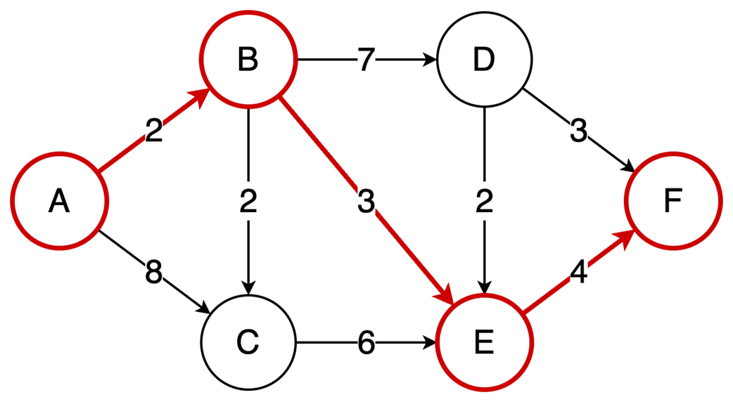
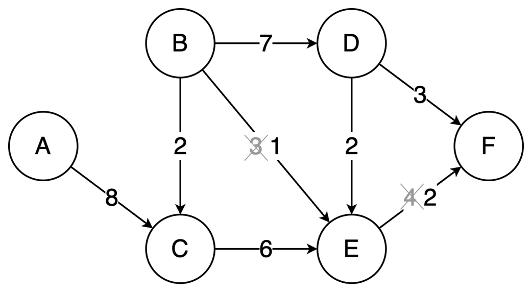
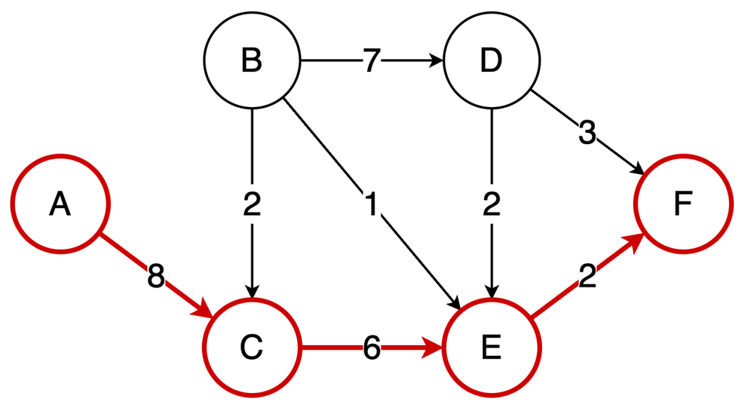
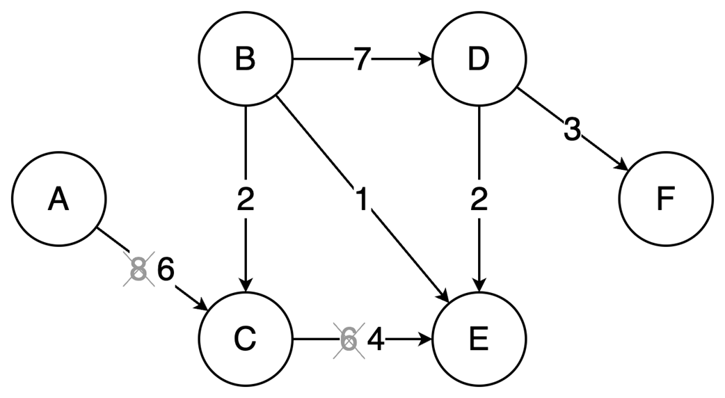
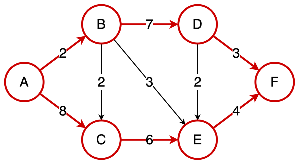
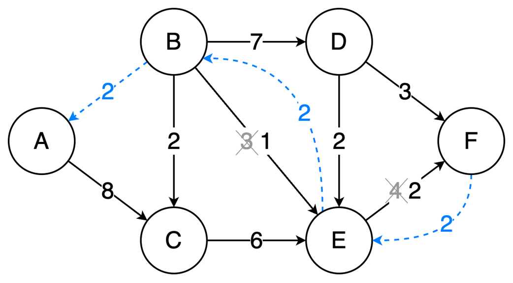
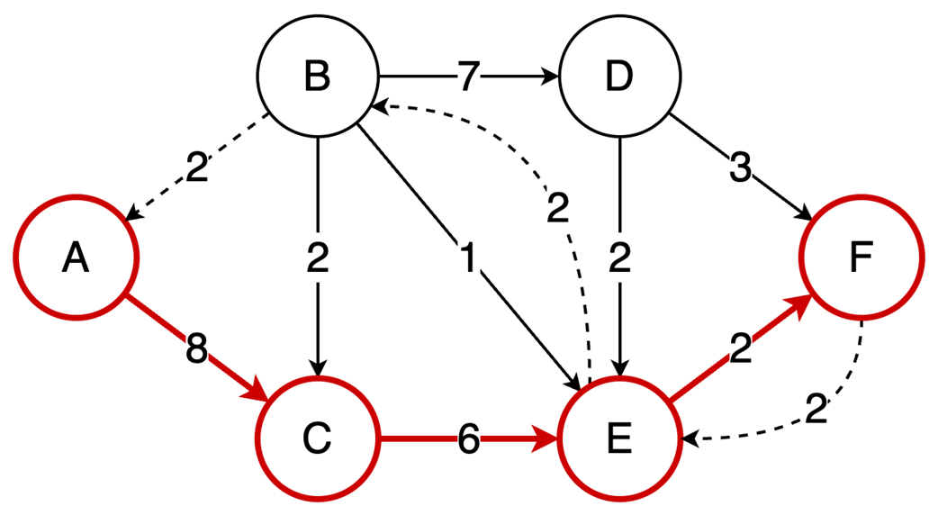
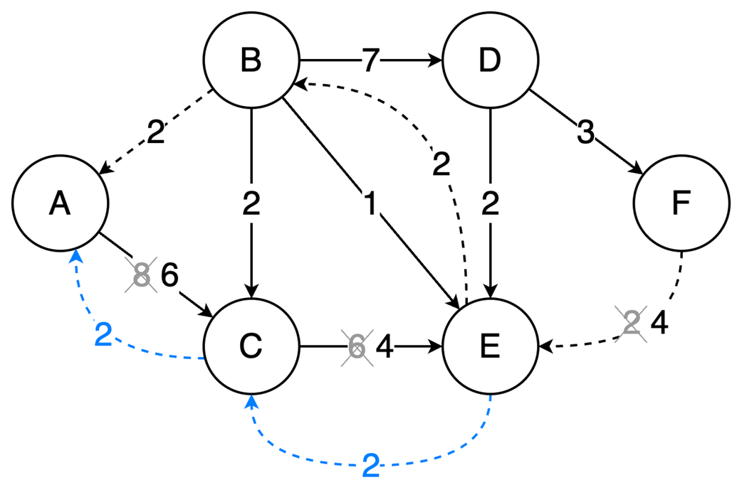
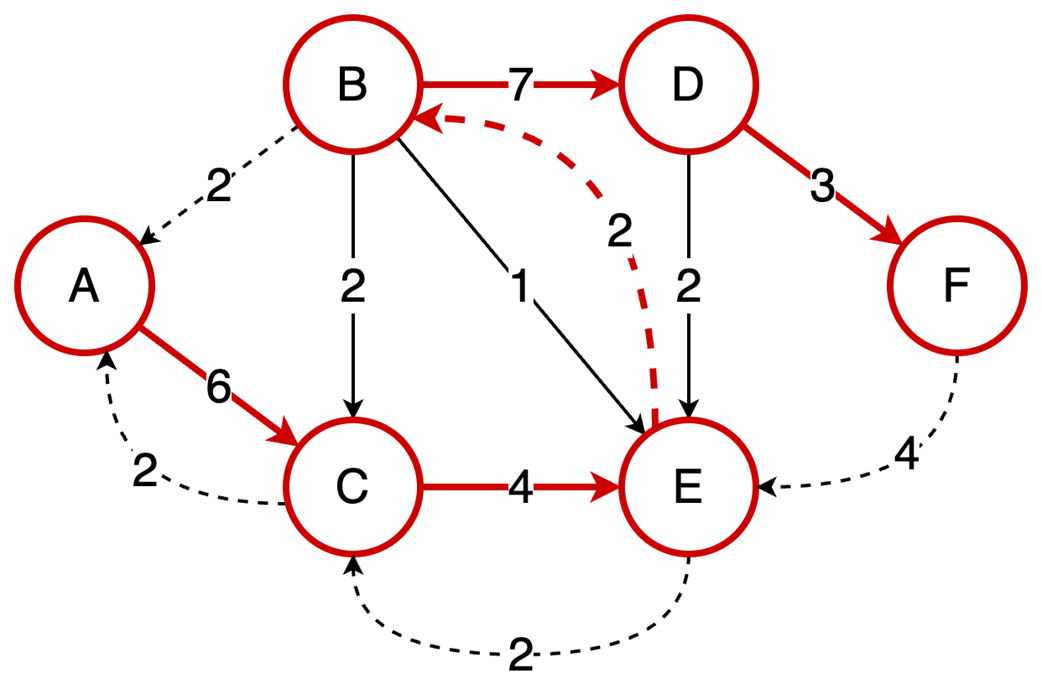
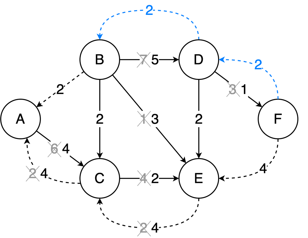
The Ford-Fulkerson algorithm solves maximum flow problems: It iteratively finds augmenting paths to push flow from source to sink and utilizes backward edges to redistribute flow, correcting suboptimal path choices.
FAQ
What is the main difference between arrays and linked lists?Arrays store elements contiguously in memory, which gives them fast index-based access and good cache locality. Linked lists store elements as nodes connected by pointers, so their elements are not guaranteed to be next to each other in memory. This makes linked lists more flexible for certain insertions and deletions, but usually worse for random access and iteration performance.When should I use a linked list instead of an array?Use a linked list when your primary operations involve frequent insertions or deletions that are not at the end of the collection, especially if you already have a reference to the insertion or deletion point. If you need fast indexed access, efficient iteration, or better cache performance, an array or dynamic array is usually a better choice.Why can linked lists be slower than arrays even when their Big-O complexity looks better?Linked lists often suffer from poor spatial locality because their nodes may not be stored contiguously in memory. This can cause more CPU cache misses. Their pointer-following access pattern is also less predictable, which makes CPU prefetching less effective. As a result, iterating over a linked list can be significantly slower than iterating over an array in practice.What is a binary heap used for?A binary heap is used when you need quick access to either the minimum or maximum element in a collection. It is commonly used to implement priority queues, where each element has a priority and the highest- or lowest-priority item must be retrieved efficiently.What are the main properties of a binary heap?A binary heap has two key properties. First, it is a complete binary tree, meaning all levels are full except possibly the last, which is filled from left to right. Second, it satisfies the heap property: in a min-heap, each parent is smaller than its children; in a max-heap, each parent is larger than its children.What are the time complexities of common heap operations?For a heap with n elements, insert takes O(log n), getMin or getMax takes O(1), and extractMin or extractMax takes O(log n). Building a heap from an unsorted array can be done in O(n) using heapify down.How are graphs commonly represented in memory?Graphs are commonly represented using either an adjacency matrix or an adjacency list. An adjacency matrix is a two-dimensional array where a[i][j] indicates whether an edge exists from vertex i to vertex j. An adjacency list maps each vertex to a list of its outgoing edges.When should I use an adjacency matrix versus an adjacency list?Use an adjacency matrix when you need very fast edge lookup, because checking whether an edge exists is O(1). However, it uses O(v²) space, so it can waste memory for sparse graphs. Use an adjacency list when the graph is sparse, because it uses O(v + e) space, though edge lookup takes O(d), where d is the degree of a vertex.What problem does topological sort solve?Topological sort produces a valid ordering of vertices in a Directed Acyclic Graph, or DAG. It is especially useful for dependency problems, such as determining package installation order, build order in tools like GNU Make, or detecting cycles that may indicate deadlocks.How does the Ford-Fulkerson algorithm solve max flow problems?Ford-Fulkerson repeatedly finds an augmenting path from a source to a sink, calculates the path’s bottleneck capacity, pushes that amount of flow through the path, and updates the residual graph. It also creates backward edges so flow can be redistributed if earlier path choices were suboptimal. The algorithm stops when no augmenting path remains, and the accumulated flow is the maximum flow.
pro $24.99 per month
access to all Manning books, MEAPs, liveVideos, liveProjects, and audiobooks!


 The Coder Cafe ebook for free