9 Running Monte Carlo simulations

Monte Carlo simulations use random sampling to approximate the behavior of complex systems when analytical solutions are impractical. The chapter introduces the core idea—simulate many possible outcomes by drawing from specified probability distributions—and contrasts this approach with deterministic models that provide single-point forecasts. It emphasizes handling both discrete and continuous random variables, the importance of defining appropriate distributions, and the value of summarizing results with probabilities and statistics to quantify uncertainty, support scenario analysis, and improve decision-making under risk.

Through a hands-on discrete example, the chapter walks step by step from defining a Poisson distribution for employee absenteeism to computing cumulative probabilities, mapping outcomes to random-number intervals, generating random samples, running trials, and interpreting results. A small, manual run (10 trials) illustrates mechanics and the pitfalls of small samples; automation then scales to 500 simulations, normalizes probabilities, and produces stable outcome frequencies that inform staffing decisions (e.g., choosing between cost efficiency and higher service levels). The discussion highlights reproducibility with random seeds, the role of expected value versus simulated variability, and why larger trial counts reduce the influence of anomalies while still reflecting rare events according to their probabilities.

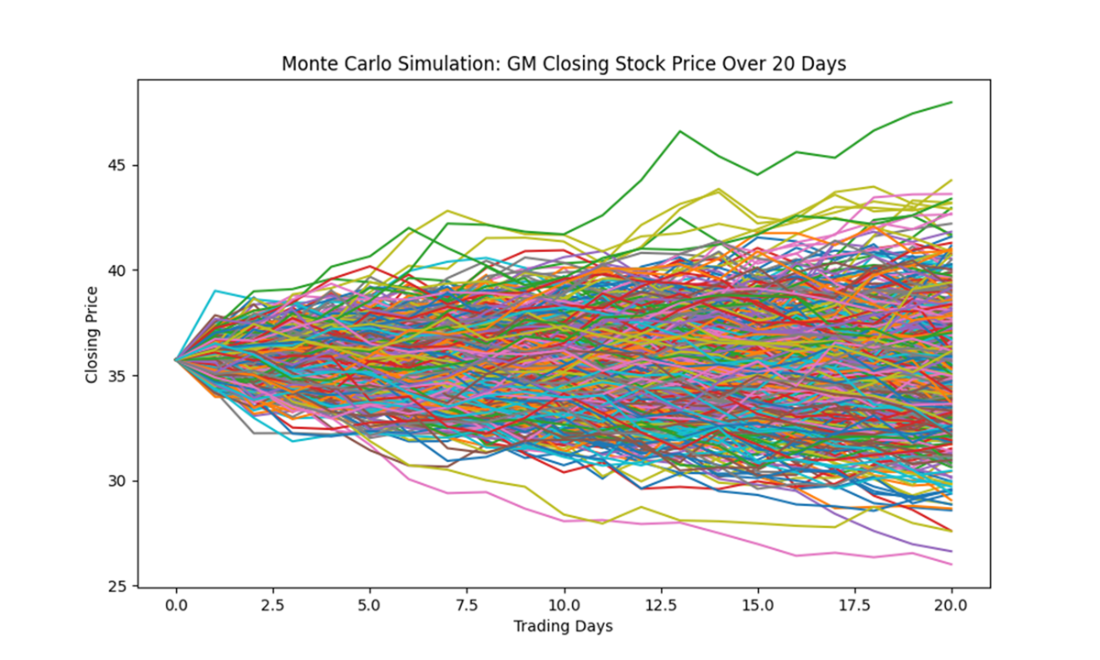
For continuous data, the chapter applies Monte Carlo methods to forecast stock prices: gather historical prices, compute daily log returns, estimate mean and volatility, draw random returns from a normal model, and iteratively compound from the last observed price to generate many price paths over a chosen horizon. Analysis of simulated paths covers directionality (ending above/below start), summary statistics across all simulated prices, and practical insights such as clustering around central tendencies, widening uncertainty over time, and the inclusion of extreme scenarios for risk assessment. The chapter concludes that Monte Carlo methods complement theory with realistic variability, offer flexible scenario exploration, and provide a robust foundation for data-driven choices in uncertain environments.

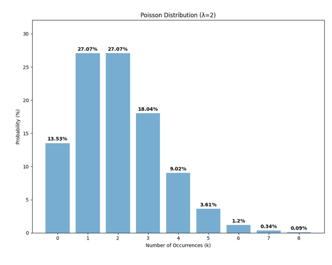
A Poisson distribution with a rate parameter (𝜆) of 2. At lower rate parameters, the distribution is right-skewed, indicating that smaller outcomes are more likely while larger outcomes become increasingly rare.

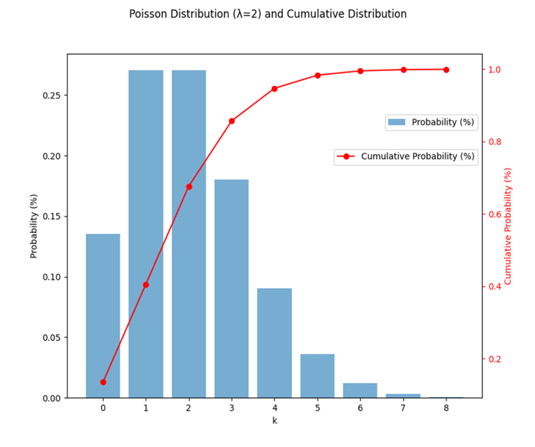
A Poisson distribution and its cumulative distribution, with the bars representing the Poisson probabilities and the line representing the cumulative probabilities. The bars correspond to the primary y-axis on the left, while the line with circular markers corresponds to the secondary y-axis on the right.

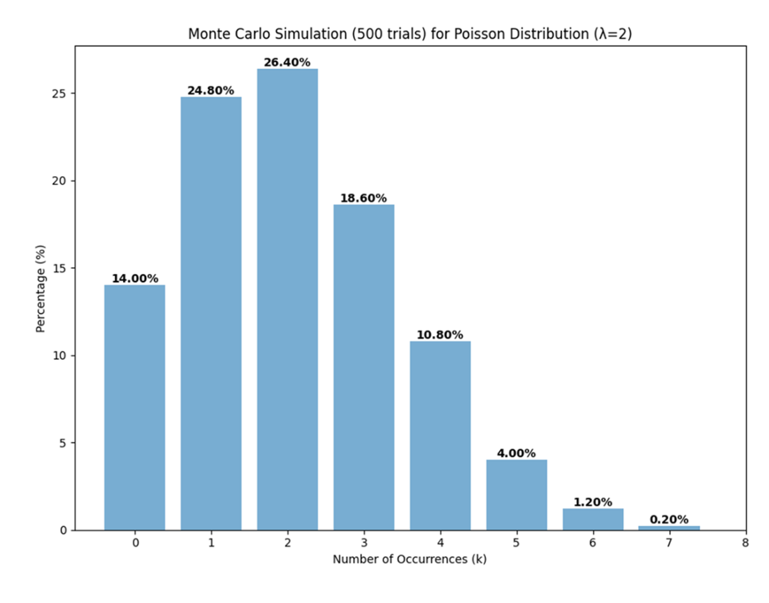
Probability distribution from 500 Monte Carlo simulations closely resembling a theoretical Poisson distribution with a rate parameter of 2. The labels atop the bars represent the percentage of trials that resulted in each unique random variable between 0 and 7. No trials results in a 𝑘 value of 8, consistent with the low theoretical probability of such an outcome.

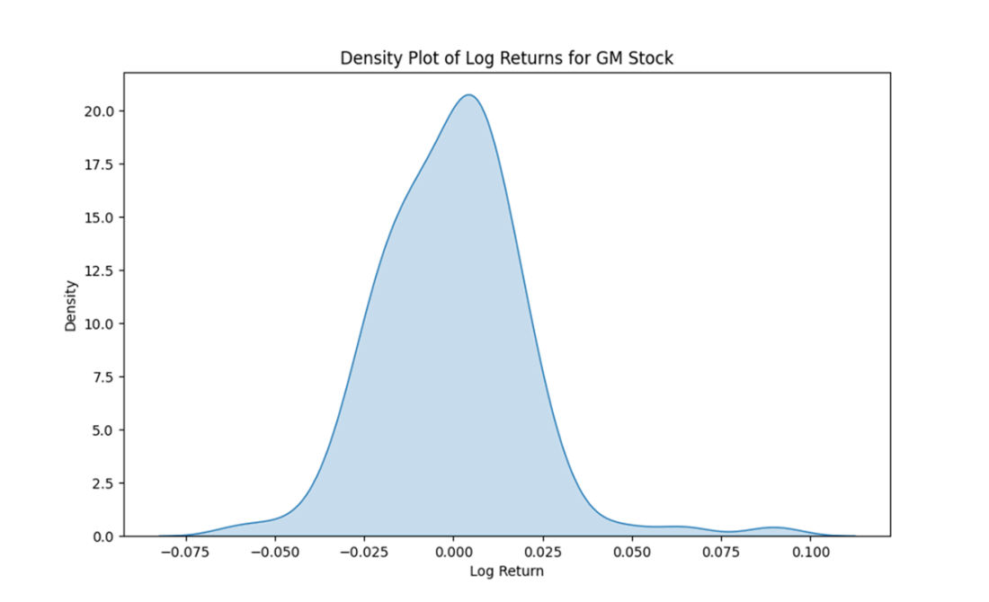
Density plot of the log returns for GM stock between July and December 2023. The distribution is approximately normal, centered around a mean close to zero, with most log returns clustered near zero but with some larger positive and negative values in the tails.

500 Monte Carlo simulations of GM’s closing stock price for January 2024. Each line represents a single trial. Each line corresponds to a single simulation, depicting potential stock price trajectories based on the historical mean and volatility of log returns.

• Monte Carlo simulations provide a powerful tool for modeling and analyzing complex systems with inherent uncertainty, offering insights into the range of possible outcomes and their probabilities. This chapter demonstrated how to apply Monte Carlo simulations to both discrete and continuous data, highlighting the differences in approach and the specific steps involved in each case.
• For discrete data, such as employee absenteeism, simulations relied on historical frequencies and discrete probability distributions to generate potential scenarios. For continuous data, such as stock price movements, the process involved calculating key statistical parameters like the mean and standard deviation to model the variability of outcomes.
• The simulations illustrated the importance of capturing inherent randomness and variability. Discrete simulations provided clarity in scenarios with distinct outcomes, while continuous simulations accounted for the fluidity of real-world processes. The chapter also emphasized the role of visual tools, such as density plots and trajectory graphs, in interpreting simulation results and understanding the implications of variability.
• Running a large number of simulations was highlighted as essential for achieving robust results, smoothing out anomalies, and providing reliable insights. By generating a range of potential future outcomes, Monte Carlo simulations empower decision-makers to assess risks, plan for contingencies, and optimize strategies in uncertain environments.
• The hands-on approach demonstrated in this chapter underscored the versatility of Monte Carlo methods in addressing both discrete and continuous uncertainties. Looking ahead, the next chapter builds on these methods, exploring decision trees to derive expected values and assess alternatives, further enhancing our capacity for data-driven decision-making.

FAQ