7 Fitting time series models

Time series modeling shifts analysis from i.i.d. data toward temporally ordered observations where trend, seasonality, and autocorrelation matter. The chapter distinguishes forecasts (future values conditioned on past order) from generic predictions, and surveys common components and use cases across finance, economics, healthcare, and digital analytics. It walks through a practical workflow—acquiring data, exploring and visualizing series behavior, and preparing features—using daily Apple closing prices as a running example to illustrate volatility, domain caveats, and the importance of respecting temporal structure when making decisions.

The ARIMA family is introduced as a unifying framework combining autoregression (AR), differencing for stationarity (I), and moving averages (MA). The chapter emphasizes assessing stationarity via visual inspection (ACF/PACF) and a formal Augmented Dickey-Fuller test, then applying first-order differencing when needed. A train/test split supports out-of-sample evaluation: an ARIMA(1,1,0) model is fitted with statsmodels, diagnostics confirm near–white-noise residuals, and forecasts are compared against April outcomes. While the approach produces reasonable estimates, the exercise highlights how market efficiency, shocks, and nonlinearity make stock-price forecasting inherently challenging and sensitive to misspecification.

Exponential smoothing offers a complementary path that directly models level, trend, and seasonality with exponentially decaying weights. The chapter contrasts Simple (SES), Double/Holt (DES), and Holt-Winters variants, then fits Holt-Winters to the same series and compares information criteria with the ARIMA fit. In this case, Holt-Winters achieves lower AIC/BIC and slightly more accurate April forecasts, underscoring that model choice should be data-driven and validated. The chapter closes by stressing diagnostics, comparative metrics, and the practicality of ensembling or model competition, all while acknowledging limits of historical-pattern extrapolation—especially in volatile domains—yet reaffirming the broad utility of these methods beyond finance.

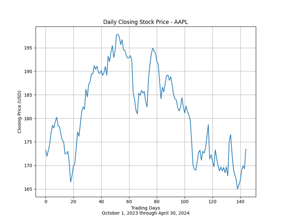
The daily closing price of Apple (AAPL) stock between October 1, 2023, and April 30, 2024. The more volatility in time series data, stock prices or otherwise, the more challenging it is to fit an accurate forecast.

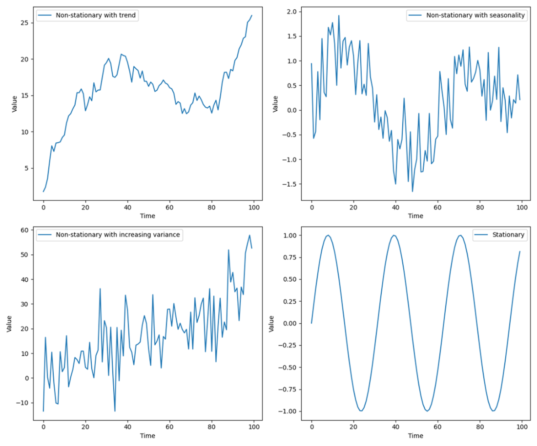
Four illustrative time series charts. Three of the subplots display non-stationary data; the fourth plot, located in the lower-right quadrant, by contrast displays stationary time series data.

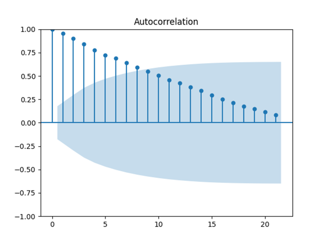
An ACF plot showing the correlation of a time series with its own past values (lags). The vertical lines represent the autocorrelation coefficients for different lags, with the blue shaded area indicating the confidence interval. Values outside this shaded region suggest significant autocorrelation, indicating a pattern in the data that could be leveraged for time series forecasting. The gradual decline in the bars signifies the "memory" effect of the time series, where past values influence future observations.

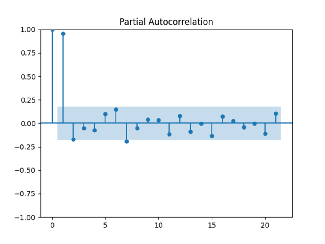
A PACF plot showing the correlation between a time series and its own past values (lags), controlling for the effects of earlier lags. The vertical lines represent the partial autocorrelation coefficients for each lag, with the blue shaded area indicating the confidence interval. Values outside this shaded region suggest significant partial autocorrelation, which can help identify the appropriate number of autoregressive terms in a time series model. The sharp drop after the first few lags indicates that only the first few lags have a significant direct effect on the current value of the series.

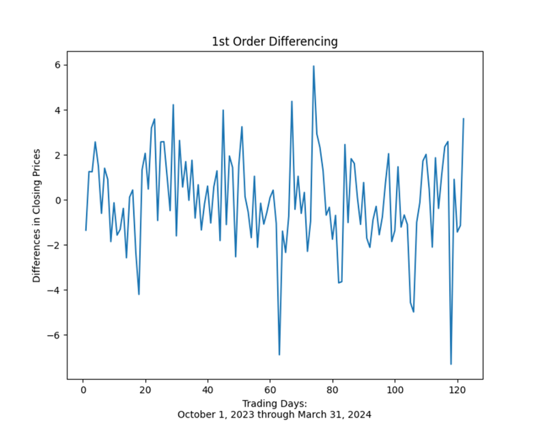
A Time series data that was converted from non-stationary to stationary by first-order differencing

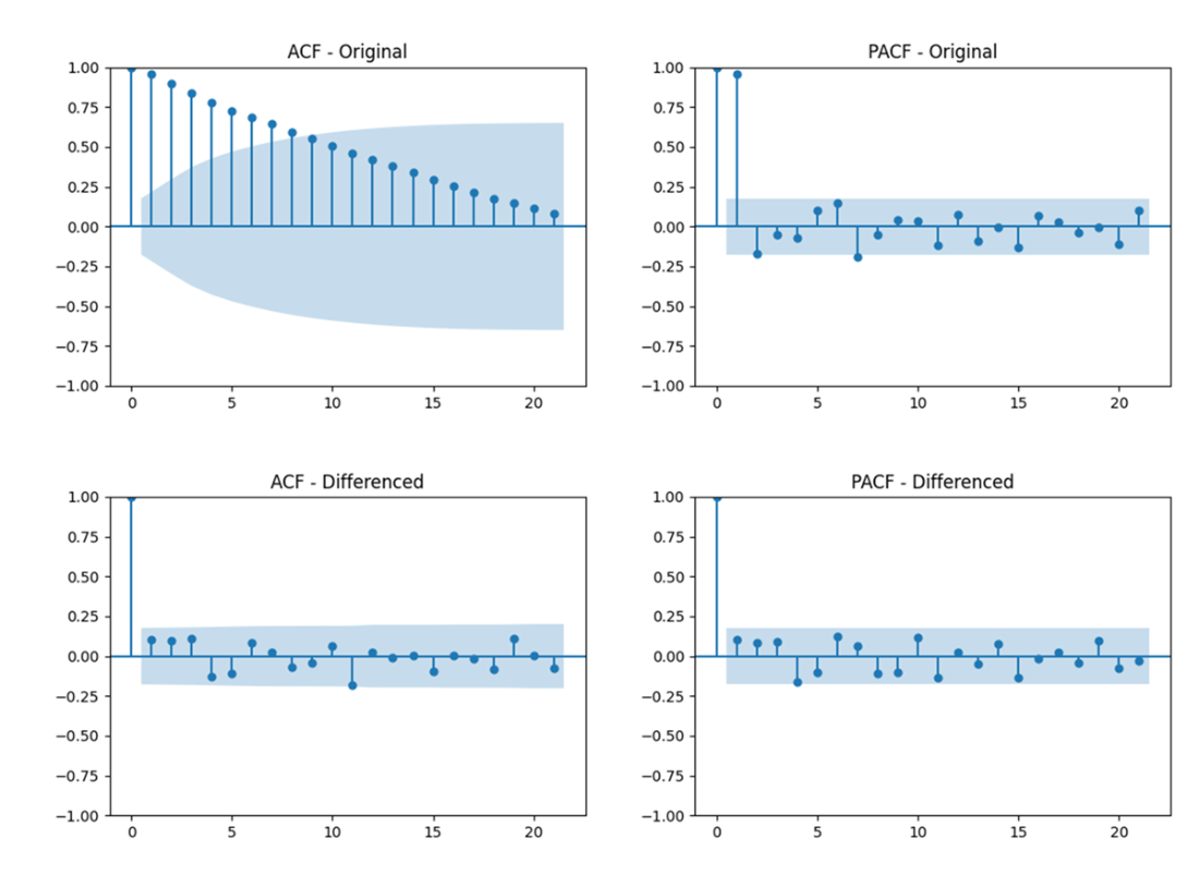
ACF and PACF plots for the original time series (top row) and first-order differenced time series (bottom row). The left column displays the ACF, showing how each observation is correlated with its previous values, while the right column presents the PACF, illustrating the direct effect of each lag. These plots are provided to compare the impact of first-order differencing on the time series’ correlation structure.

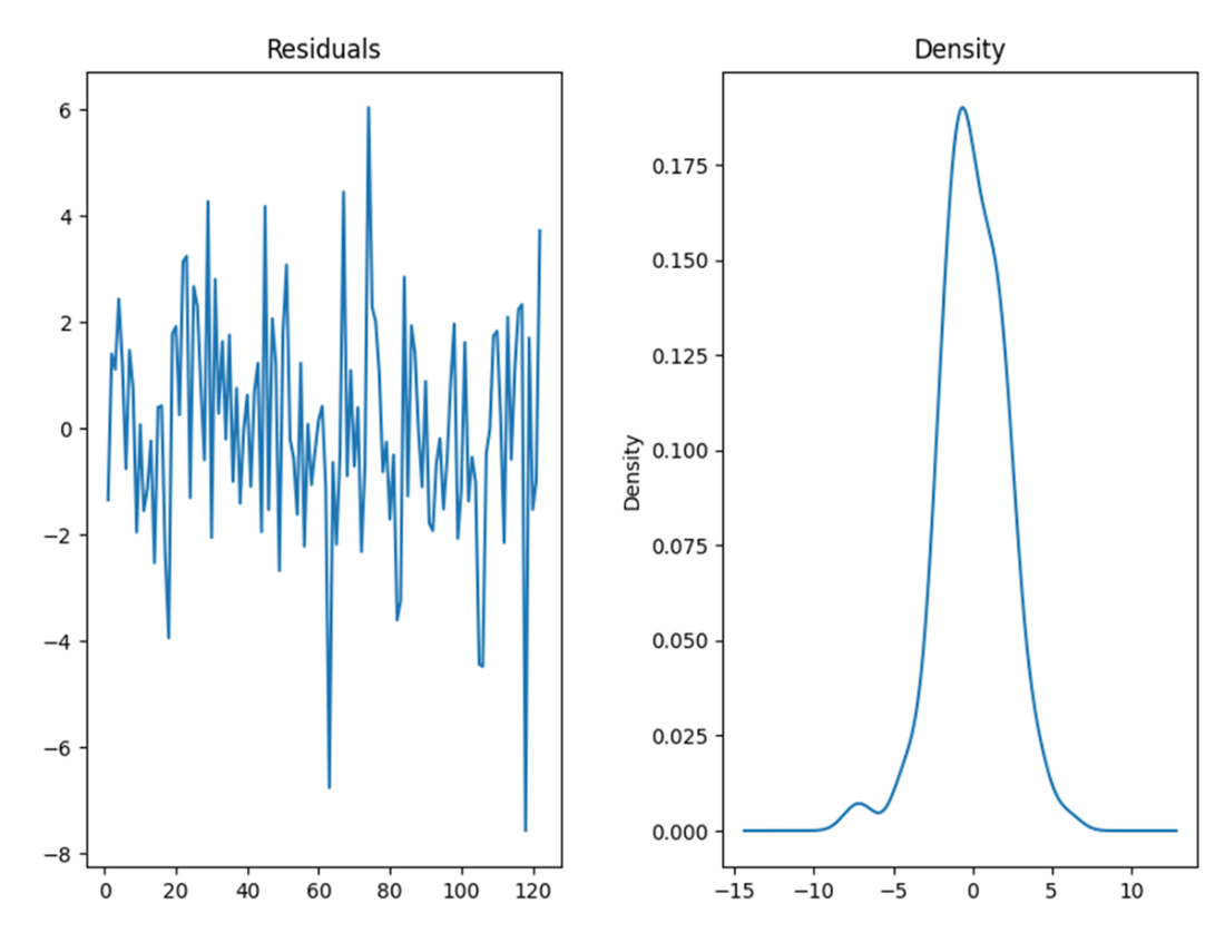
On the left, the model residuals display no obvious pattern or trend; on the right, the same residuals are normally distributed around a mean of zero.

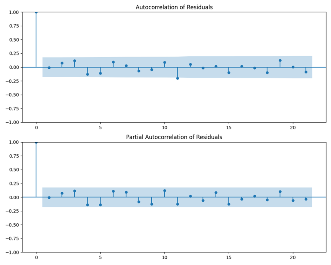
ACF plot (on the top) and PACF plot (on the bottom) of the model residuals. The lack of statistically significant correlations further suggests that the ARIMA model sufficiently captured trends in the time series.

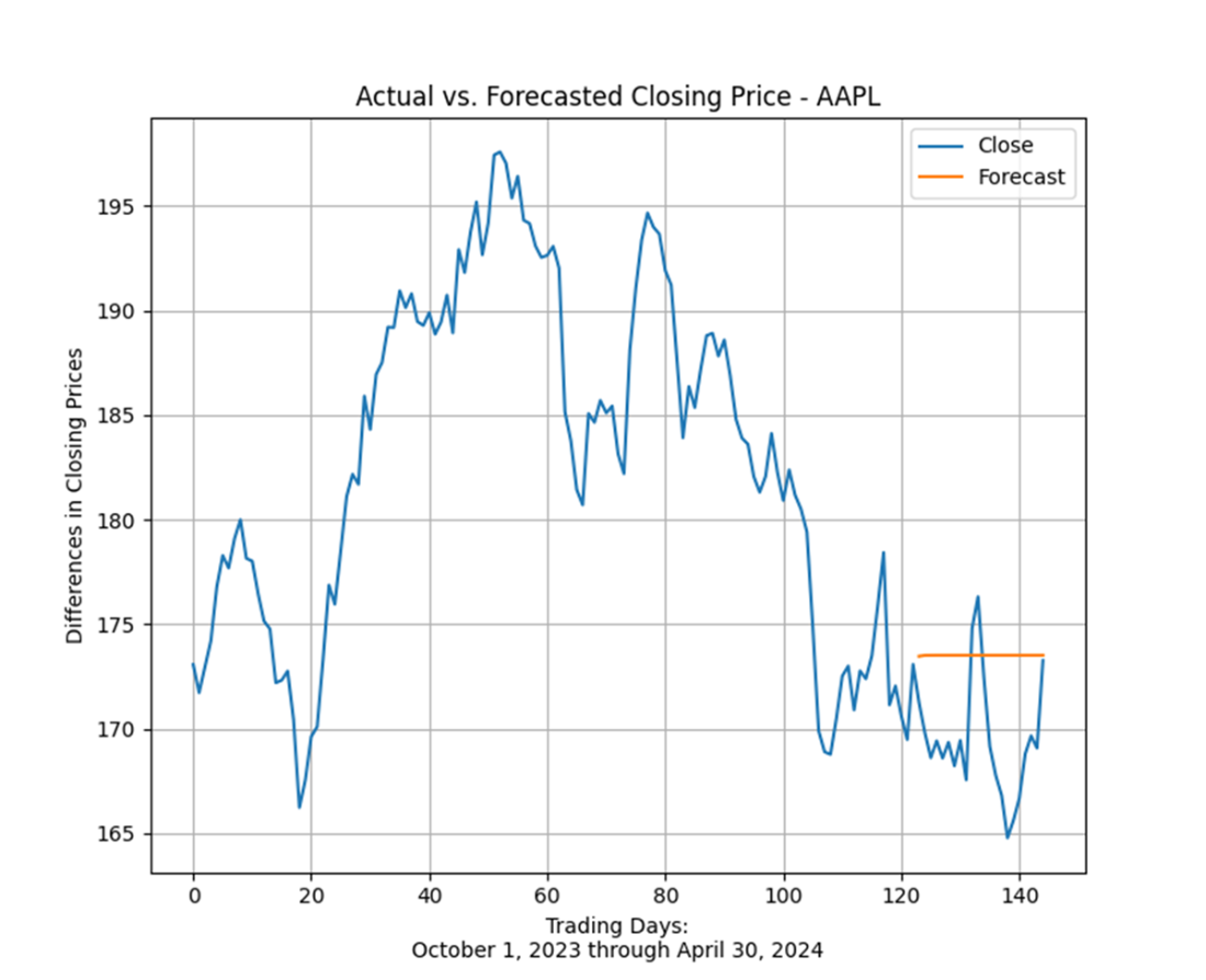
The actual closing prices of Apple stock from October 1, 2023, through April 30, 2024, plus the forecasted closing price of the stock throughout April 2024 generated from an ARIMA model.

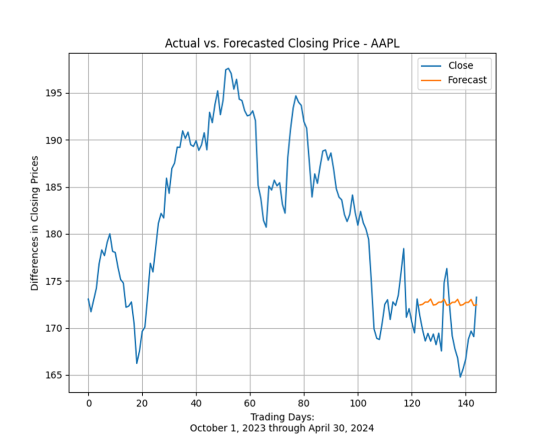
The actual closing prices of Apple stock from October 1, 2023, through April 30, 2024, plus the forecasted closing price of the stock throughout April 2024 generated from a Holt-Winters exponential smoothing model. The Holt-Winters exponential smoothing forecast is slightly more accurate than the forecast from our ARIMA model.

• A time series model is a statistical tool used to understand and predict the behavior of data points indexed by time. It analyzes patterns and trends within sequential data, aiming to capture dependencies and variations over time. Time series models typically account for seasonality, trends, and irregular fluctuations in data, making them essential for forecasting future values or understanding historical patterns.
• ARIMA (AutoRegressive Integrated Moving Average) is a popular time series forecasting model that combines autoregressive (AR), differencing (I), and moving average (MA) components. ARIMA models are versatile for handling a wide range of time series data by capturing its temporal structure, seasonality, and trend. The AR component models the relationship between an observation and a lagged value, while the MA component models the dependency between an observation and a residual error from a moving average model. The differencing component handles non-stationary data by transforming it into a stationary series.
• Exponential smoothing models do not require as much preprocessing as ARIMA models because they primarily focus on smoothing past data to make forecasts. They do not involve complex parameter determination through differencing or identifying autoregressive and moving average components, as ARIMA models do. This simplicity in preprocessing makes exponential smoothing models easier and quicker to implement for forecasting time series data with less historical analysis and adjustment.
• Simple Exponential Smoothing is a forecasting technique that assigns exponentially decreasing weights to past observations. It is suitable for time series data without trends or seasonal patterns. SES is characterized by its reliance on a single smoothing factor, which controls the rate of decay of older observations. Despite its simplicity, SES can provide effective short-term forecasts by emphasizing recent data over historical values.
• Double Exponential Smoothing extends simple exponential smoothing by incorporating a trend component into the forecasting process. In addition to the smoothing parameter for level smoothing, DES introduces a trend smoothing parameter. This model is suitable for time series data exhibiting a trend but no seasonal pattern. DES forecasts are influenced by both recent observations and the trend observed in previous periods, making it more robust than simple exponential smoothing for data with a linear trend.
• Holt-Winters Exponential Smoothing extends double exponential smoothing by adding a seasonal component to handle time series data with seasonal variations. It therefore includes three smoothing parameters: level smoothing, trend smoothing, and seasonal smoothing. This model is effective for forecasting data with both trend and seasonal patterns, providing a flexible approach to capture and forecast seasonal variations in time series data.

FAQ