6 Fitting a decision tree and random forest

This chapter introduces tree-based models for classification and regression, focusing on how to fit, interpret, and evaluate decision trees and random forests. It frames the ideas with a realistic prediction task: whether an NFL team converts a fourth down. The workflow emphasizes practical data preparation and exploration—filtering to relevant plays, handling missing values, transforming score differential to reflect the offense’s perspective, encoding categories, and deriving the binary target (CONVERT) from yards gained versus yards to go. Exploratory analysis highlights which features are most informative, notably that shorter “to-go” distances strongly correlate with success, play type aligns with the yardage required, and quarter and score context offer secondary signals. Throughout, the chapter balances model building with interpretation, evaluation, and the trade-offs between simplicity, accuracy, and robustness.

The decision tree section explains recursive partitioning, split criteria (Gini impurity or entropy), stopping rules, pruning, and how to read node attributes. It shows a complete pipeline: selecting features (quarter, to-go, venue, score differential, play type), creating train/test splits, fitting a depth-limited classifier, making predictions, and assessing performance. The fitted tree achieves about 61% accuracy overall, with markedly better performance on successful conversions than failures, illustrating class-dependent behavior. Interpretation ties back to the data: the root split is at TO_GO ≤ 3.5, reflecting that short distances dominate outcomes; subsequent splits involve PLAY_TYPE, SCORE_DIFFERENTIAL, and venue, refining predictions while reducing impurity. The chapter also walks through the math of Gini impurity—how to compute it for categorical and numeric features, weight impurities across child nodes, and choose thresholds by scanning midpoints—making clear why TO_GO emerges as the most discriminative variable.

The random forest section builds on this foundation, describing how bagging (bootstrap sampling) and random feature selection at each split reduce variance and mitigate overfitting relative to a single tree. Using a modest forest (50 shallow trees), the model edges up to about 62% accuracy overall, again performing substantially better on successful conversions than failures. Feature importance ranks TO_GO and PLAY_TYPE as dominant, with quarter and score adding smaller but meaningful contributions; sampling individual trees from the ensemble reveals diverse structures and split choices. The chapter closes by contrasting advantages and drawbacks: decision trees are transparent and easy to deploy but can overfit and be unstable; random forests trade some interpretability for robustness and improved generalization. Together, these methods give programmers practical, statistically grounded tools for interpretable modeling and stronger predictive performance.

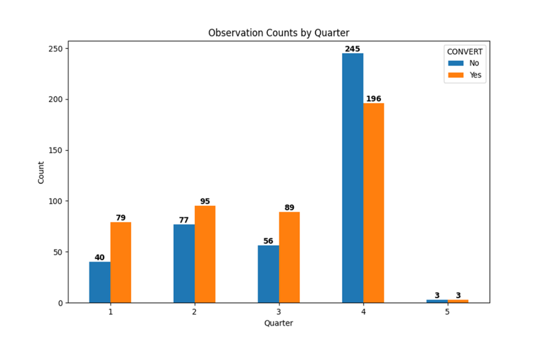
A grouped bar chart that displays the CONVERT class label counts by QUARTER. Teams were more successful than not converting fourth down attempts in the first three quarters, but less successful in the fourth quarter.

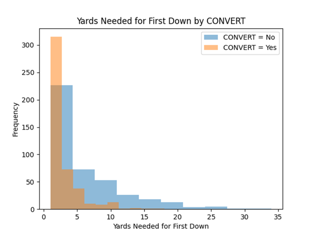
Paired histograms that display the distributions of TO_GO grouped by the CONVERT class labels. When teams succeeded on their fourth down attempts, they usually needed less than 3 yards to convert, and definitely fewer than 5 yards. When teams failed to convert on fourth down, they oftentimes needed to gain more than 5 yards, and sometimes up to 25 yards or more.

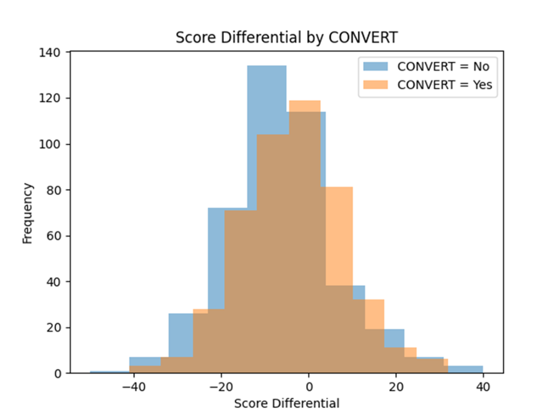
Paired histograms that display the distributions of SCORE_DIFFERENTIAL grouped by the CONVERT class labels. Regardless of the CONVERT class label, the distribution is normally distributed about the mean.

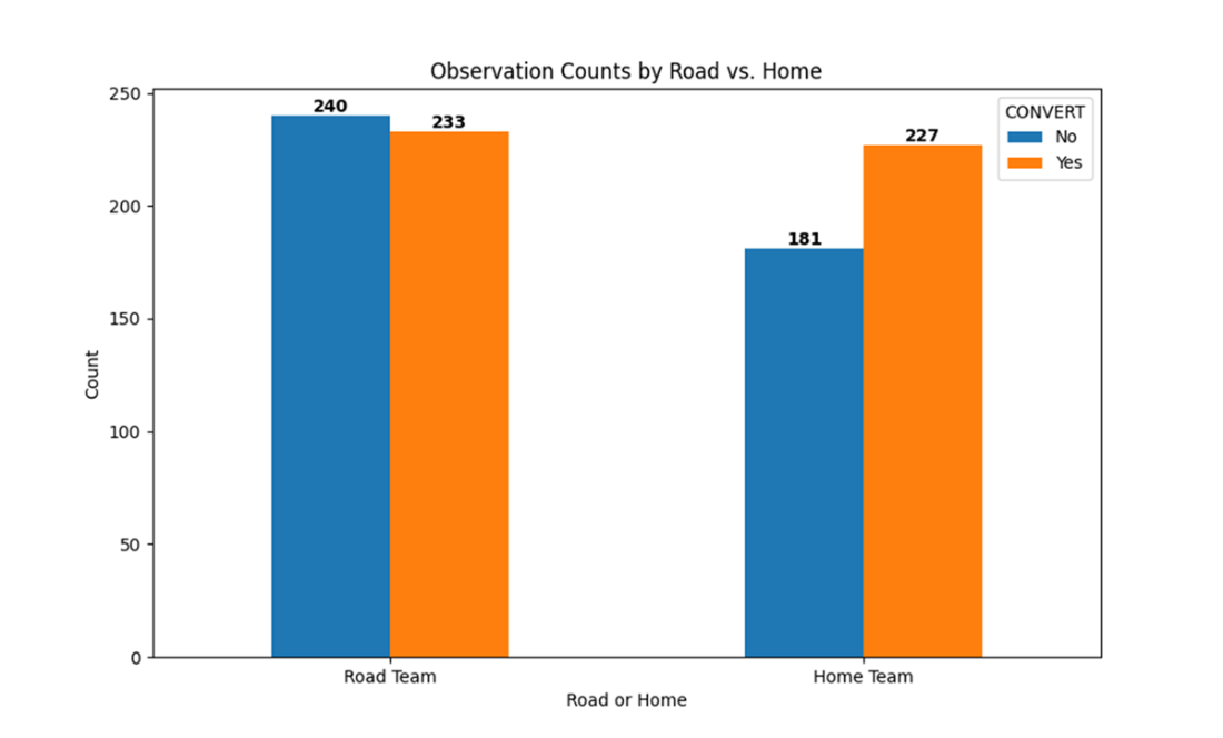
Counts of fourth down conversion attempts categorized by the OFFENSIVE_TEAM_VENUE and CONVERT class labels. Teams playing at home were more successful than visiting teams in converting fourth down attempts.

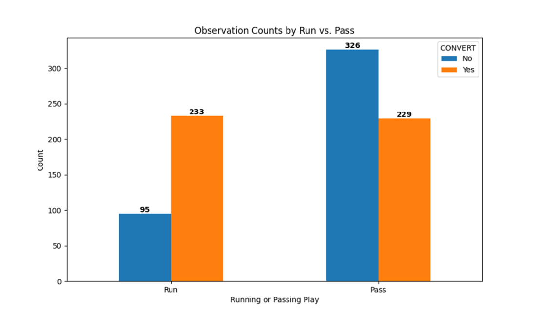
Counts of fourth down conversion attempts categorized by the PLAY_TYPE and CONVERT class labels. Teams that ran the ball on fourth down were much more successful in converting those attempts compared to other teams that passed the ball instead. This doesn’t necessarily mean that running is typically a better strategy than passing; rather, it might simply reflect the yards required for a conversion.

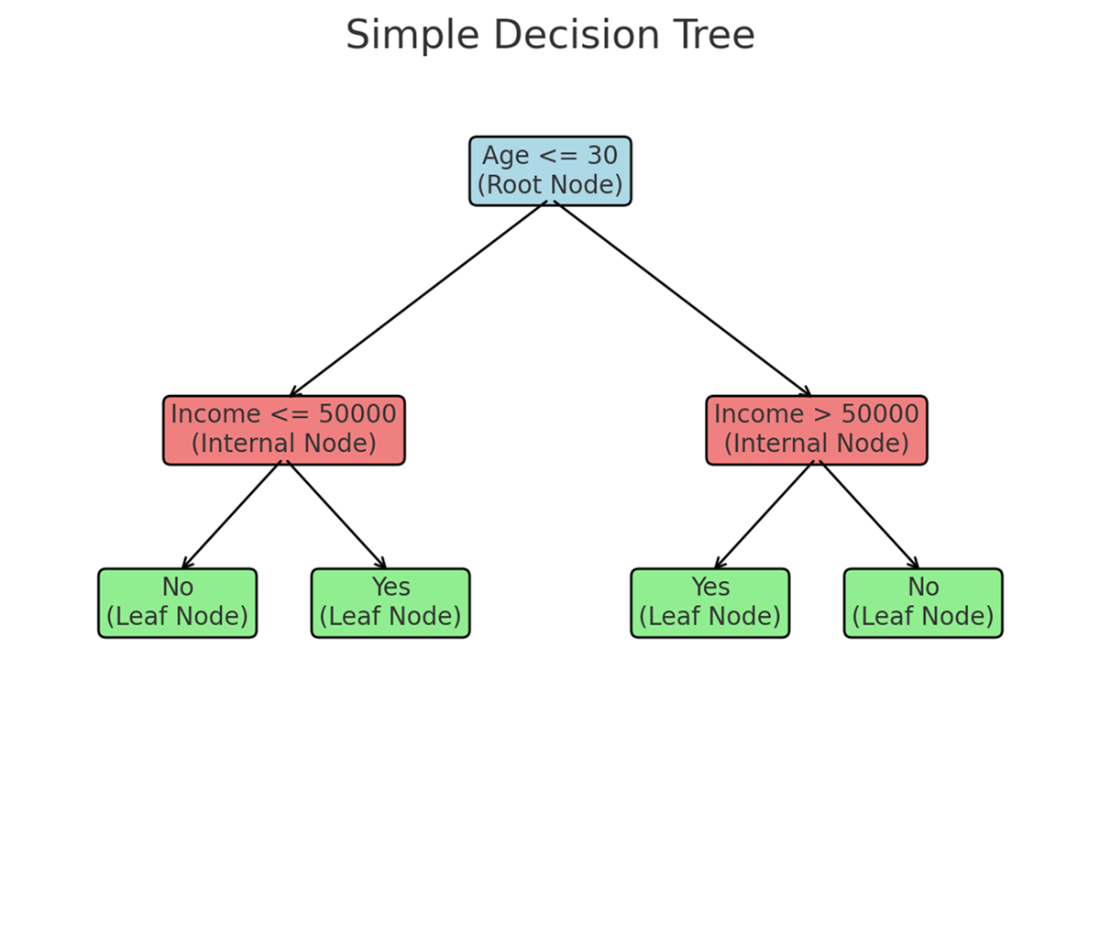
A decision tree demonstrating the home loan approval process based on the applicant’s age and income. The tree is interpreted from top to bottom, starting at the root node and progressing to the leaf nodes. The left branch is followed when conditions are true, and the right branch is followed when conditions are false.

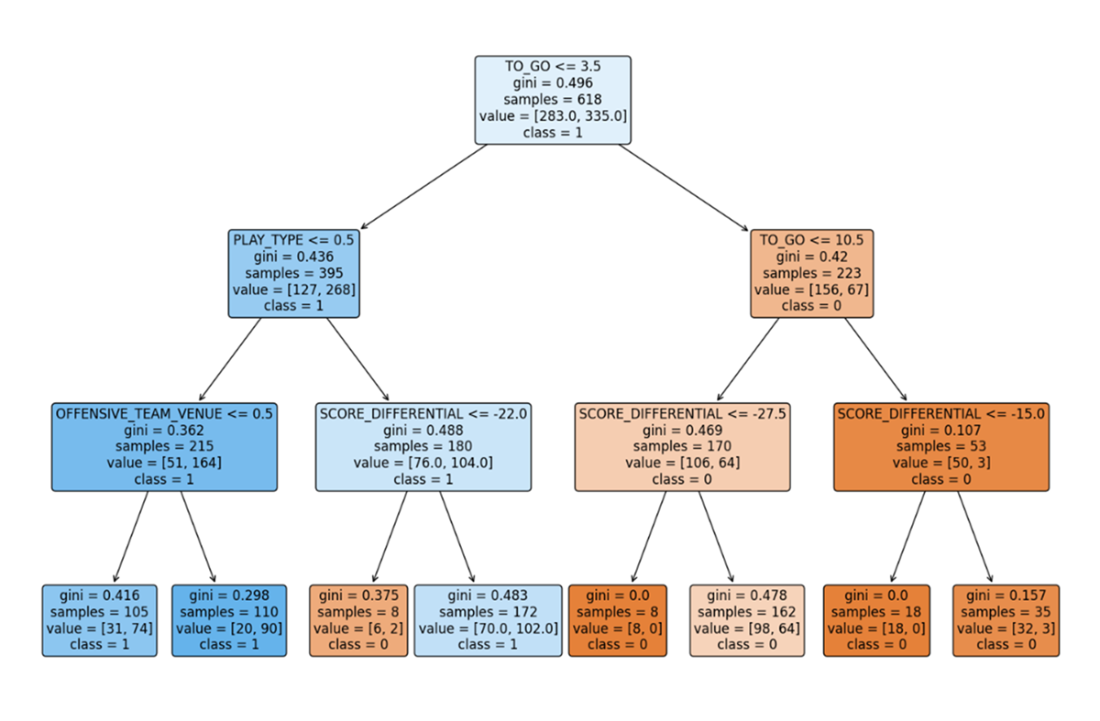
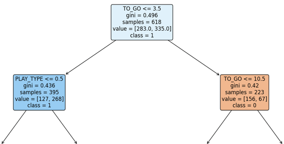
A plotted decision tree that represents the model’s decision-making process, showing how features are used to split the data and make predictions. This tree was pruned during construction, so it contains fewer splits and even fewer (less significant) features than otherwise.

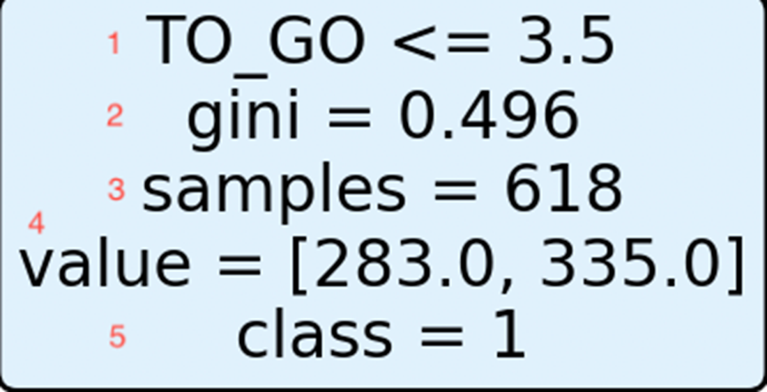
A close look at the root node attributes from the plotted decision tree. The root node and the internal nodes all contain these same attributes; leaf nodes have these same attributes, too, minus the condition statement at the top.

A close look at the very top of our decision tree—the root node and the first level of internal nodes. The root node has arrows pointing away from it, while internal nodes have arrows pointing toward and away from them.

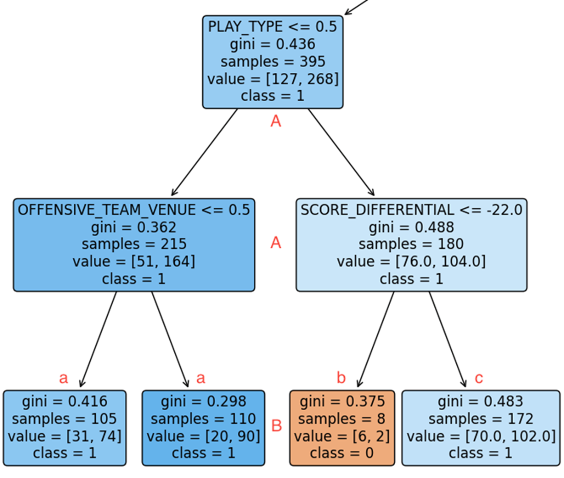
A closer look at the left subtree—two levels of internal nodes (A) and, at the bottom, four leaf nodes (B). When PLAY_TYPE is 0, thereby indicating a running play, the decision tree predicts a successful fourth down conversion attempt (a); it doesn’t matter if the team on offense is the road or home team. Alternatively, when PLAY_TYPE is 1, indicating a passing play, the decision tree then evaluates SCORE_DIFFERENTIAL before making a prediction. If the team on offense is trailing by 22 points or more, the tree predicts a failed fourth down conversion attempt (b); but if the team on offense is trailing by fewer than 22 points, the decision tree predicts a successful conversion (c).

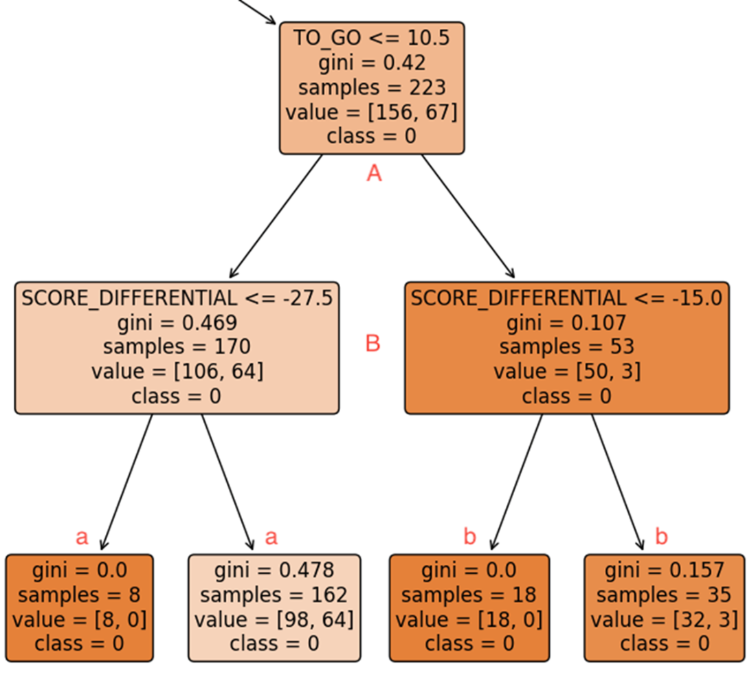
The right branch of the decision tree uses internal nodes TO_GO (A) and SCORE_DIFFERENTIAL (B) to establish a classification pathway, with the initial TO_GO split playing a crucial role in distinguishing the target class, followed by subsequent refinements that confirm the predicted class labels (a and b).

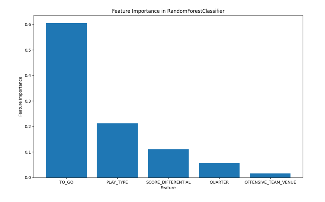
A feature importance plot generated from the RandomForestClassifier. It displays the relative importance of each feature to the final predicted class labels where, if stacked, a single bar would equal 1. The features are otherwise sorted, from left to right, in descending order of relative importance, with TO_GO and PLAY_TYPE accounting for approximately 80% of the model’s predictive power.

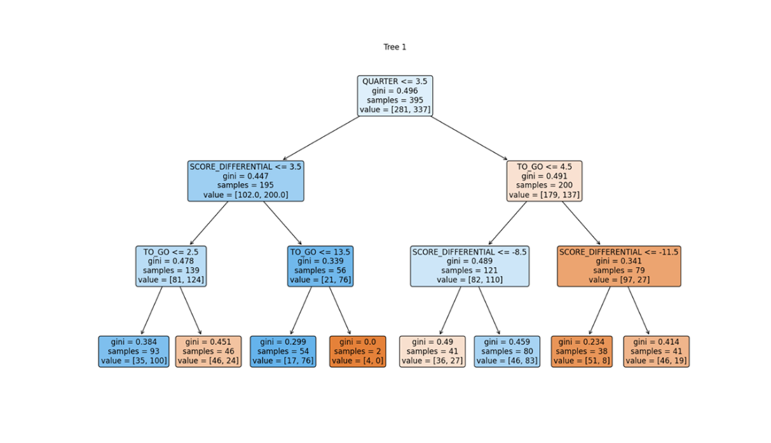
The first of two random trees from a random forest model containing 50 trees. Notice that QUARTER is at the root node; thus, based on this one random split of the data, QUARTER, which didn’t factor into our decision tree model, is the most significant variable in this subset for predicting the final class labels.

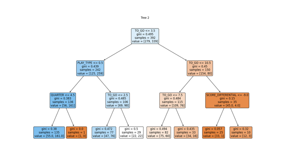
The second of two random trees from the same random forest model. The features and splits to construct one tree versus another can, and will, vary significantly.

• A decision tree is a supervised machine learning model used for classification and regression tasks. It splits the data into subsets based on feature values, creating a tree structure with decision nodes and leaf nodes representing predictions. Decision trees are easy to interpret and visualize.
• Training a decision tree involves splitting the data based on features to minimize node impurities. It uses the training set for learning and the test set for evaluation, ensuring unbiased accuracy and generalization assessment.
• Evaluating a decision tree includes computing overall accuracy by comparing predicted and actual labels in the test set. A confusion matrix provides a detailed performance breakdown, showing true/false positives and negatives for each class, helping to identify areas for improvement.
• Building a decision tree involves recursive splitting based on significant features to maximize class separation, continuing until the subsets are pure or meet stopping criteria. Interpretation follows the path from root to leaves, ensuring consistent model construction and understanding.
• A random forest is a supervised model for classification and regression, consisting of multiple decision trees trained on different data and feature subsets. This ensemble method typically enhances accuracy and reduces overfitting by aggregating predictions from multiple trees, providing robust performance.
• Evaluating a random forest involves steps similar to a decision tree, including computing overall accuracy and using a confusion matrix for granular performance insights. The aggregated results from multiple trees offer a more robust evaluation and reliable performance across classes.
• Feature importance in random forests measures each feature's contribution to predictive power by assessing impurity reduction across all trees. This provides a comprehensive view of influential features, helping to identify and prioritize significant variables for accurate predictions.
• While this chapter focuses on decision trees and random forests, other powerful tree-based methods like XGBoost and Gradient Boosting are also popular for tackling complex classification and regression problems. These models build on the strengths of decision trees, using advanced techniques to boost accuracy and handle challenging data patterns, offering further options for sophisticated analysis beyond what we covered here.

FAQ