4 Fitting a linear regression
This chapter presents linear regression as a core supervised learning technique for predicting numeric outcomes and answering practical questions programmers care about: whether a meaningful relationship exists between predictors and a response, its direction and strength, how to quantify expected changes, which variables matter in multiple regression, how well the model fits, and whether assumptions are satisfied. It distinguishes simple from multiple regression, frames the model as a line of best fit through data, and motivates its enduring value across domains such as marketing, housing, admissions, and retail forecasting. The treatment combines conceptual grounding with an end‑to‑end, hands‑on workflow to build, interpret, and validate a model.
On the theory side, the chapter covers the linear and multiple regression equations, ordinary least squares estimation, and residuals, then explains goodness‑of‑fit using R-squared while cautioning about its limits: it always increases with added predictors, does not imply causality, and can mask model misspecification or overfitting. It clarifies positive, negative, and neutral relationships and emphasizes conditions for best fit, notably the influence of non-normality and outliers. Practical remedies are discussed—data transformations (log, reciprocal, square root, modest power) and outlier handling (removal or winsorization)—with the warning that such steps alter the modeling scale, may hide nonlinearity better addressed by other methods, and should be justified and documented.
On the practice side, readers import and explore a small race‑timing dataset with pandas, compute descriptive statistics, test variable normality via Shapiro–Wilk, and screen for outliers using a three‑standard‑deviation rule. They fit an OLS model with statsmodels, interpret coefficients (intercept and slope) and predictions, and connect output back to sums of squares (SST, SSR, SSE) to derive R-squared. Model significance is evaluated with the F‑statistic and its p‑value, and individual predictors via t‑tests. Assumptions are then diagnosed: linearity (residuals plot), independence (Durbin–Watson), homoscedasticity (Breusch–Pagan), and residual normality (Q–Q plot and Jarque–Bera). The chapter closes by noting multicollinearity concerns in multiple regression and reinforcing a careful, transparent workflow to balance simplicity, interpretability, and generalization.
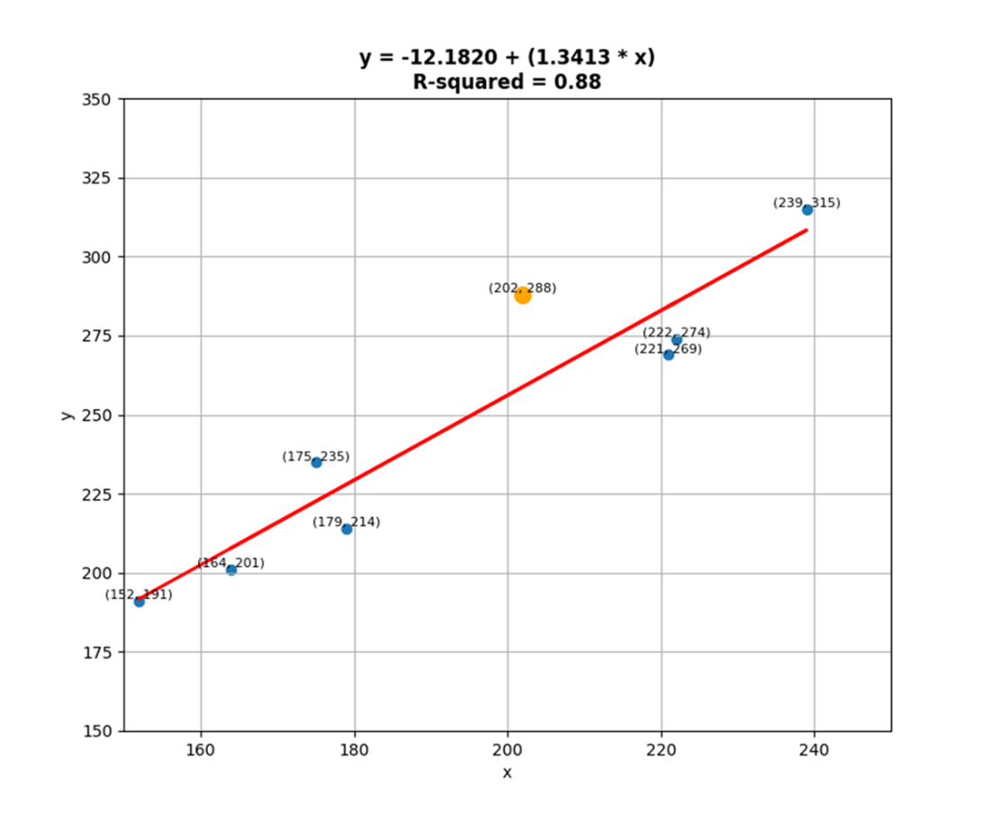
A scatter plot that displays 8 data points, their respective x and y coordinates, and a regression line. The data points represent the observed data (for instance, when x equals 202, y equals 288, which has been highlighted and magnified). The regression line ties back to a simple linear regression that was fit on the data where a response variable called y, which runs along the y-axis, was regressed against a predictor called x, which runs along the x-axis. It otherwise represents the linear equation at the top that can be derived from the model output; which is to say it is also a representation of the predictions for y given x. R-squared is one of several metrics contained in the model output; it represents the percentage of variance in the response variable that can be explained by changes in the predictor.
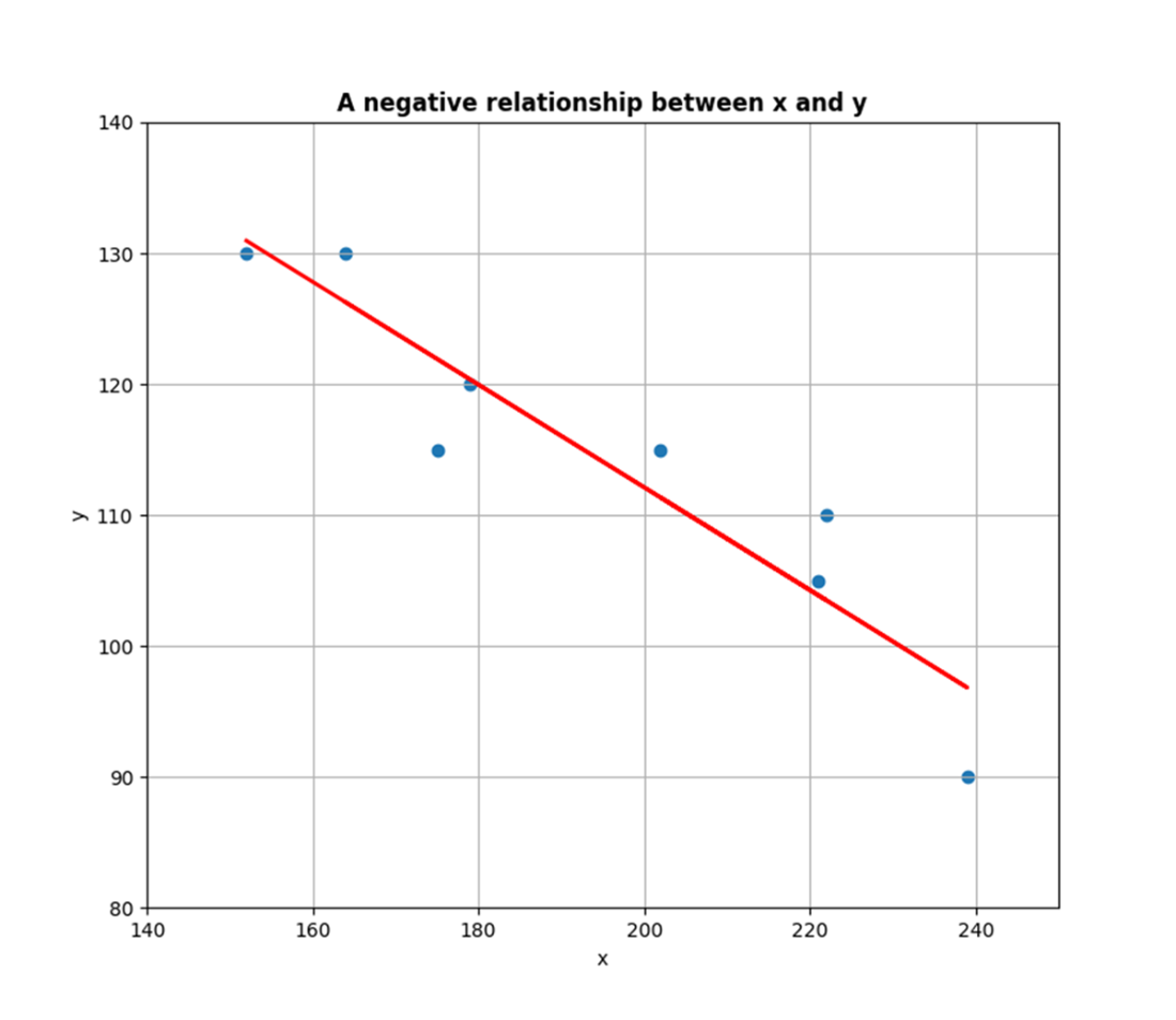
A scatter plot that shows a negative relationship between variables. The relationship is negative because the variables move in opposite directions—as the independent variable x increases, the dependent variable y decreases.
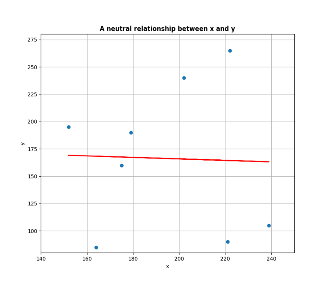
A scatter plot that shows a neutral relationship between variables. The relationship is neutral because changes in the independent variable x appear to have almost no effect on the dependent variable y.
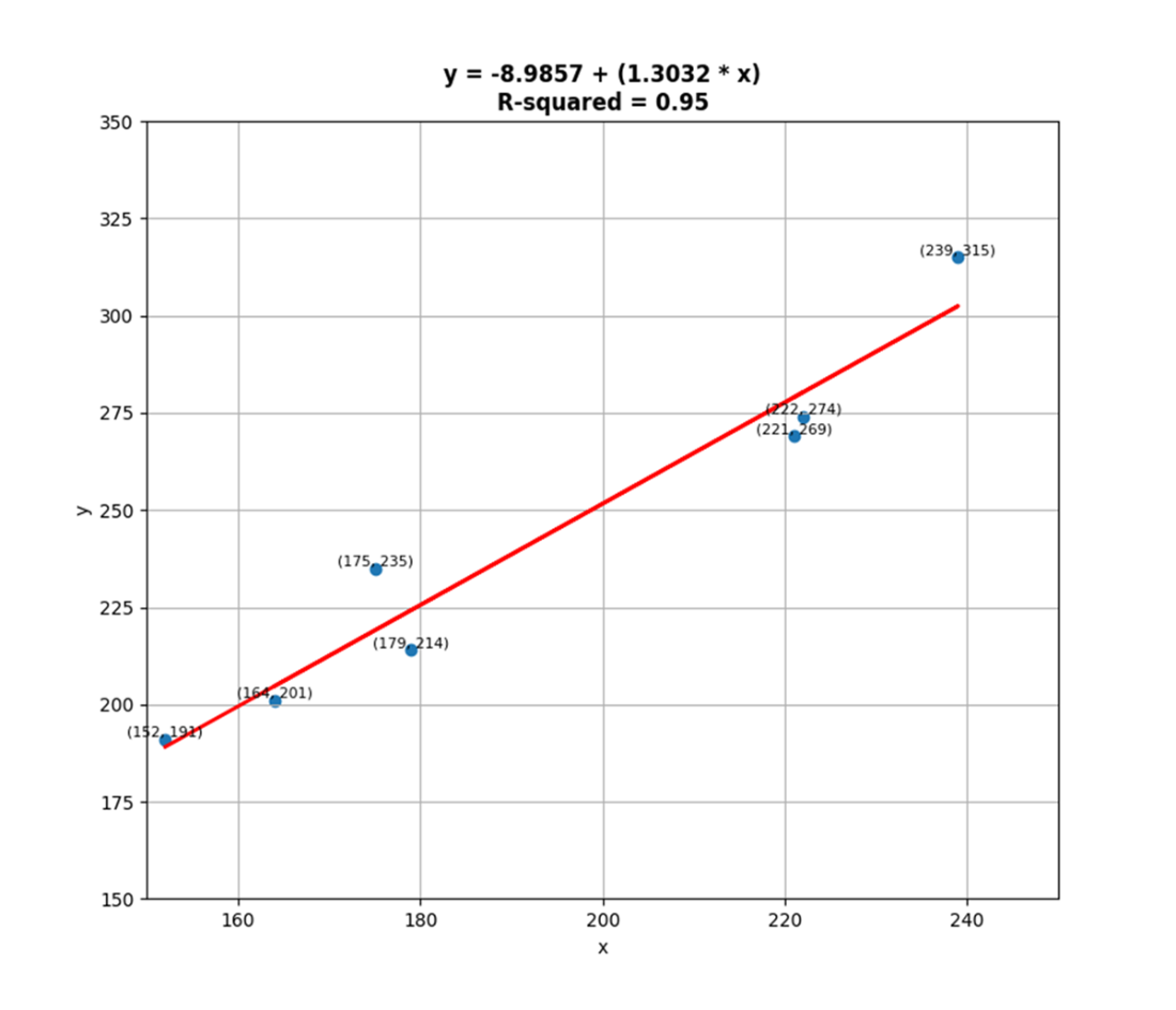
A scatter plot that displays 7 data points rather than 8. The one presumed outlier was removed and another regression was fit, resulting in a coefficient of determination now equal to 0.95, which was previously equal to 0.88. By removing one outlier, we’ve made a strong model even stronger.
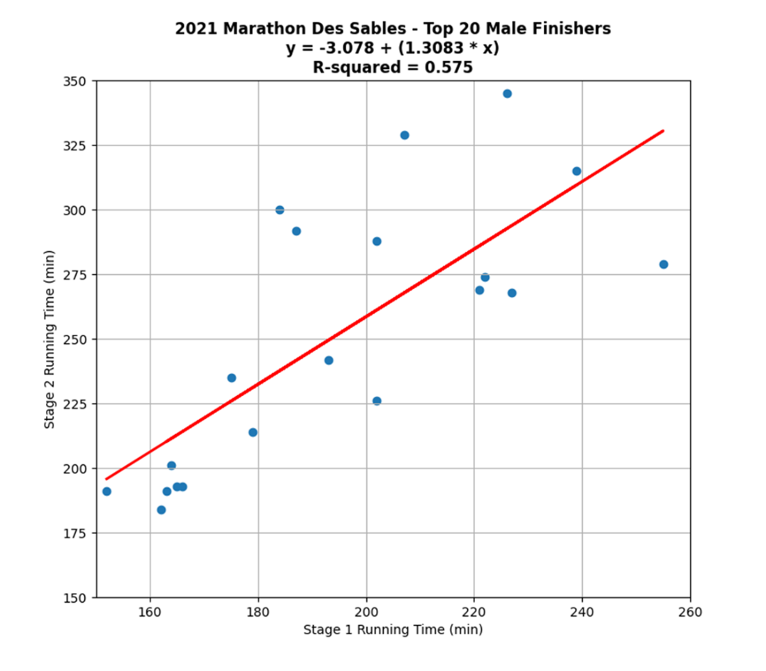
A scatter plot that displays the observed stage1 and stage2 values from the mds data frame, their respective x and y coordinates, and a regression line that represents the predictions for stage2 from a simple linear regression where stage2 was regressed against stage1. The regression line is otherwise drawn from applying the linear equation at the top of the plot. R-squared is one of several metrics contained in the model output; it represents the percentage of variance in stage2 that can be explained by changes in stage1.
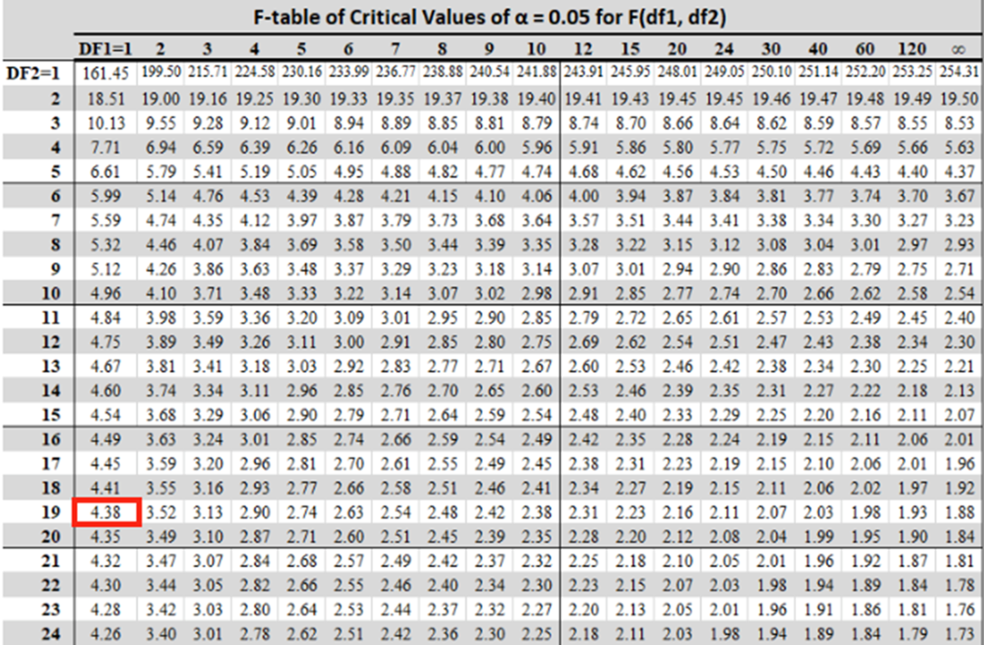
A snippet from a typical F-table where the selected significance level equals 5%. The critical value is located at the intersection of the predictor count (equal to 1) and the observation count, minus 1 (equal to 19). Because the F-statistic is greater than the critical value, the model therefore explains a statistically significant amount of the variance in the response variable.
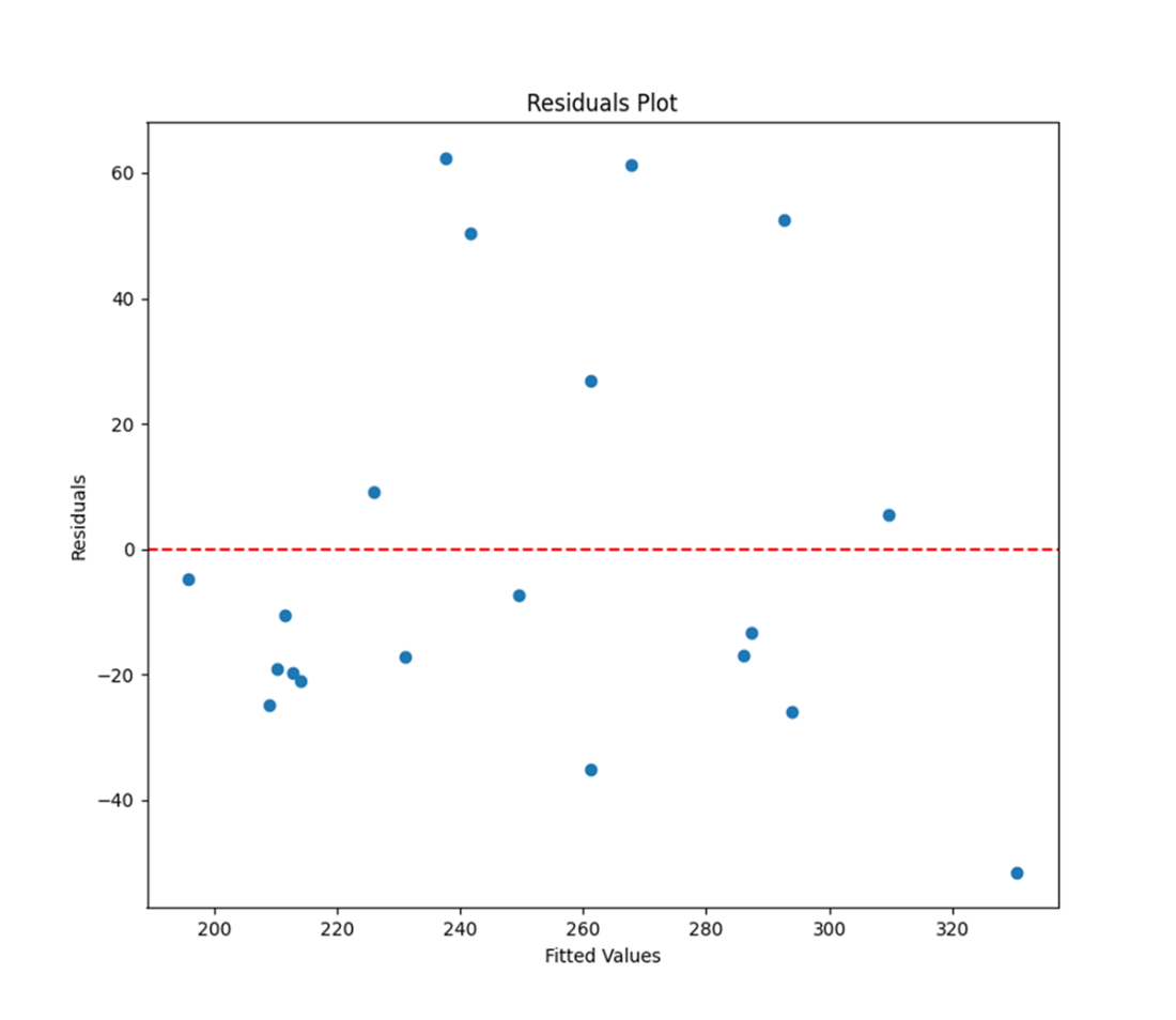
A residuals plot that displays the fitted values from a linear regression on the x-axis and the residuals from the same model on the y-axis. Linearity between variables is confirmed when the data points do not follow any obvious pattern or trend.
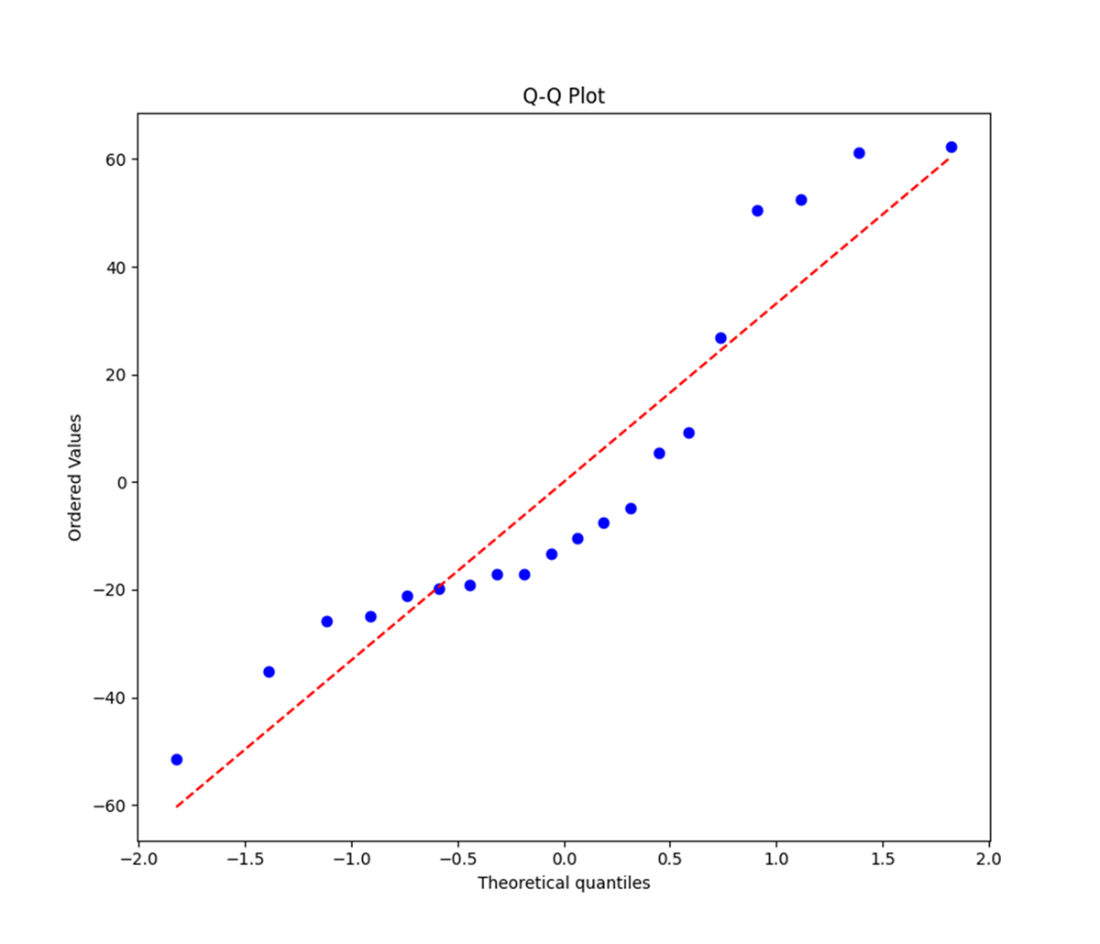
A Q-Q plot that displays the distribution of the residuals (points) versus a perfectly-normal distribution (dashed line). Linear regression assumes that the residuals are normally distributed; however, our Q-Q plot might suggest otherwise.
Summary
- Linear regression is a statistical method used to model the relationship between a numeric dependent variable and one or more independent variables by fitting a linear equation to observed data. It assumes a linear relationship between the independent and dependent variables, with the goal of estimating the parameters of the linear equation to minimize the overall difference between observed and predicted values. Linear regression is commonly used to predict and understand the relationship between variables across multiple domains, including economics, finance, and the social sciences.
- Goodness of fit should be evaluated from multiple measures. R2, or the coefficient of determination, which equals a number between 0 and 1 that specifies the proportion of variance in the dependent variable explained by the regression, might be the most meaningful measure, but hardly the only measure that matters. Overall fit is determined by the F-statistic. Significance (and insignificance) are fixed by the p-values for the individual coefficients as well as the p-value for the model.
- Testing for model assumptions—linearity between variables, independence, homoscedasticity, and normality of the residuals—warrants the reliability and validity of regression results and therefore further facilitates interpretation and decision-making.
- Applying best practices along the way, like testing for normality in the predictors and removing any and all outliers from the data, contribute considerably to getting a best possible fit and guaranteeing positive results in post-regression tests.
FAQ
When should I use linear regression, and when should I avoid it?
Use it when you want to model or predict a numeric (continuous) response from one or more predictors and the relationship is approximately linear. Do not use linear regression for classification problems; consider logistic regression or other classifiers instead.What is the basic linear regression equation and how do I interpret the coefficients?
The simple model is ŷ = β₀ + β₁x. β₀ (intercept) is the predicted value when x = 0. β₁ (slope) is the expected change in the response for a one-unit increase in x. Residuals are the differences between observed and predicted values.How do I fit a simple linear regression in Python with statsmodels?
- Define y (response) and x (predictor)- Add an intercept with sm.add_constant(x)
- Fit the model: lm = sm.OLS(y, x).fit()
- Review results: print(lm.summary())
What does R-squared tell me, and what are its limitations?
R-squared is the proportion of variance in the response explained by the predictor(s), ranging from 0 to 1. Limitations: it does not show direction or causality, it can increase just by adding predictors (even weak ones), and a high value does not guarantee linearity or good generalization. Use Adjusted R-squared to penalize unnecessary predictors.How do I interpret p-values in the output (P>|t| and Prob(F-statistic))?
- P>|t| tests each coefficient: a small p-value (e.g., < 0.05) suggests that predictor’s effect is statistically significant.- Prob(F-statistic) tests the model as a whole: a small p-value indicates the regression explains a statistically significant portion of the response variance.
What assumptions does linear regression make, and how can I test them?
- Linearity: check a residuals vs fitted plot; no pattern suggests linearity holds.- Independence of residuals: use the Durbin–Watson statistic; values near 2 suggest independence.
- Homoscedasticity (constant variance): use the Breusch–Pagan test; p-value > 0.05 suggests constant variance.
- Normality of residuals: inspect a Q–Q plot and confirm with the Jarque–Bera test.
Should I test variables for normality before modeling? How?
While the assumption applies to residuals, checking variable distributions helps. Use the Shapiro–Wilk test on predictors/response; a p-value > 0.05 suggests the data are not significantly different from normal. Normal predictors often lead to more normal residuals.How do outliers affect linear regression, and how can I handle them?
Outliers can unduly influence the fitted line and reduce model reliability. Detect them via scatter plots or rules like values beyond ±3 standard deviations. Possible treatments: transform data (log, sqrt, reciprocal), winsorize extreme values, or remove outliers with caution (risk of overfitting or bias). Always document your choices.What does the F-statistic measure, and how is it used?
The F-statistic evaluates whether the model explains significantly more variance than a model with only an intercept. You interpret it via its p-value (Prob(F-statistic)); a small value (e.g., < 0.05) indicates the model is statistically significant overall.What are SST, SSR, and SSE, and how do they relate to R-squared?
- SST (total): total variability in the response around its mean.- SSR (regression): variability explained by the model.
- SSE (error): unexplained variability (sum of squared residuals).
They relate as SST = SSR + SSE, and R-squared = SSR / SST = 1 − SSE / SST.
 Statistics Every Programmer Needs ebook for free