3 Exploring probability distributions and conditional probabilities
This chapter deepens the journey from random variables to practical reasoning under uncertainty by focusing on core probability distributions and conditional probabilities. It builds on prior fundamentals to explain how distributions model real-world phenomena and how programmers can translate those ideas into precise computations. Throughout, the text balances intuition with implementation, showing how to move smoothly between theory, visualization, and executable code.
The discussion centers on four widely used distributions. For the normal distribution, it distinguishes density from probability, highlights the 68–95–99.7 rule, and shows how to compute probabilities via standardization and the cumulative distribution function. The binomial distribution is framed as a model for repeated binary trials, with parameters n and p determining its mean and spread, and a shape that often resembles the normal distribution under common conditions; computations use the probability mass function directly or via library routines. The discrete uniform distribution emphasizes equal likelihood across a finite set and its implications for simulation and fairness. The Poisson distribution models event counts over fixed intervals using a single rate parameter λ (equal to both mean and variance), with shapes that evolve from right-skewed to approximately normal as λ grows. A companion section on probability problems reinforces essential rules—the complement rule, multiplication and addition rules, odds, permutations, and combinations—through concise, realistic exercises.
The final part introduces conditional probability as reasoning with updated information: narrowing the sample space changes the denominator and, consequently, the probability. Through accessible examples (weather, medical testing, traffic, sports, and investing), the chapter contrasts dependence with independence and demonstrates two complementary solution strategies: an intuitive contingency-table approach and the formulaic P(A|B) = P(A and B) / P(B). Programmatic workflows show how to extract counts and compute conditional probabilities directly from tabulated data. Together, these tools equip readers to compute, combine, and condition probabilities with confidence in real-world analytical settings.
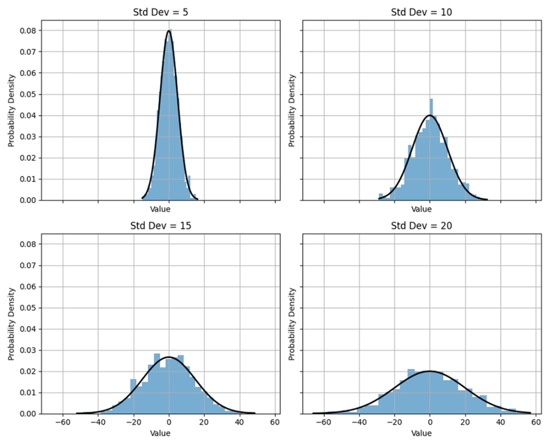
A 2 x 2 grid of normal distributions where each plot shares the same x-axis and y-axis scales. The mean equals 0 throughout and the standard deviation equals 5, 10, 15, or 20. Increases in the standard deviation translate to greater dispersion from the mean, flatter distributions, and wider tails. In other words, the probability density function becomes more dispersed across a larger range of values, and the distribution is broader and less peaked around the mean. The bell-like shape applies throughout, however, where the values are distributed symmetrically around the mean.
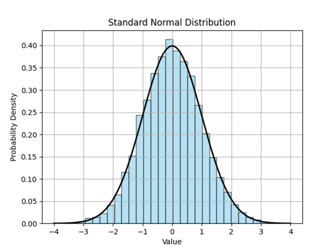
A standard normal distribution is a normal distribution where the mean is equal to 0, the standard deviation is equal to 1, and the values have been standardized from their raw form. The probability density function typically peaks at or around 0.399.
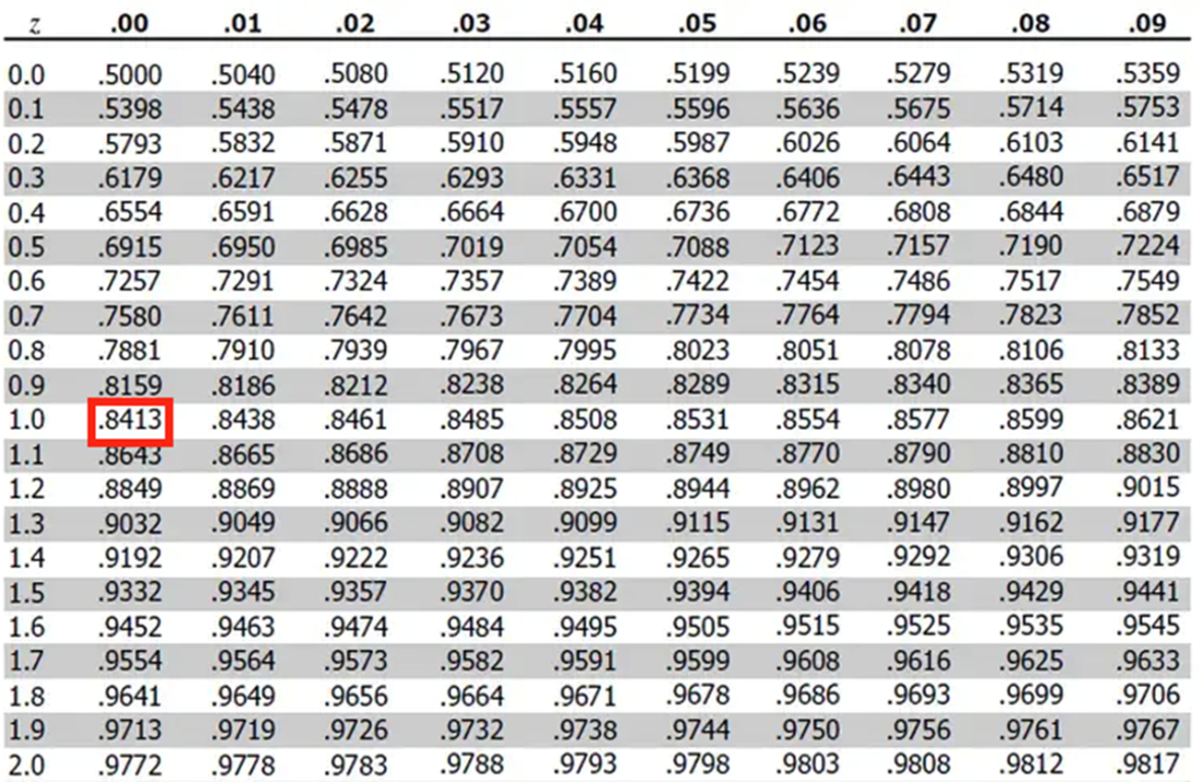
The top of a typical z-score table. The probability (or area to the right of a particular value that has been standardized) is found where the integer and remaining fractional parts of the value intersect.
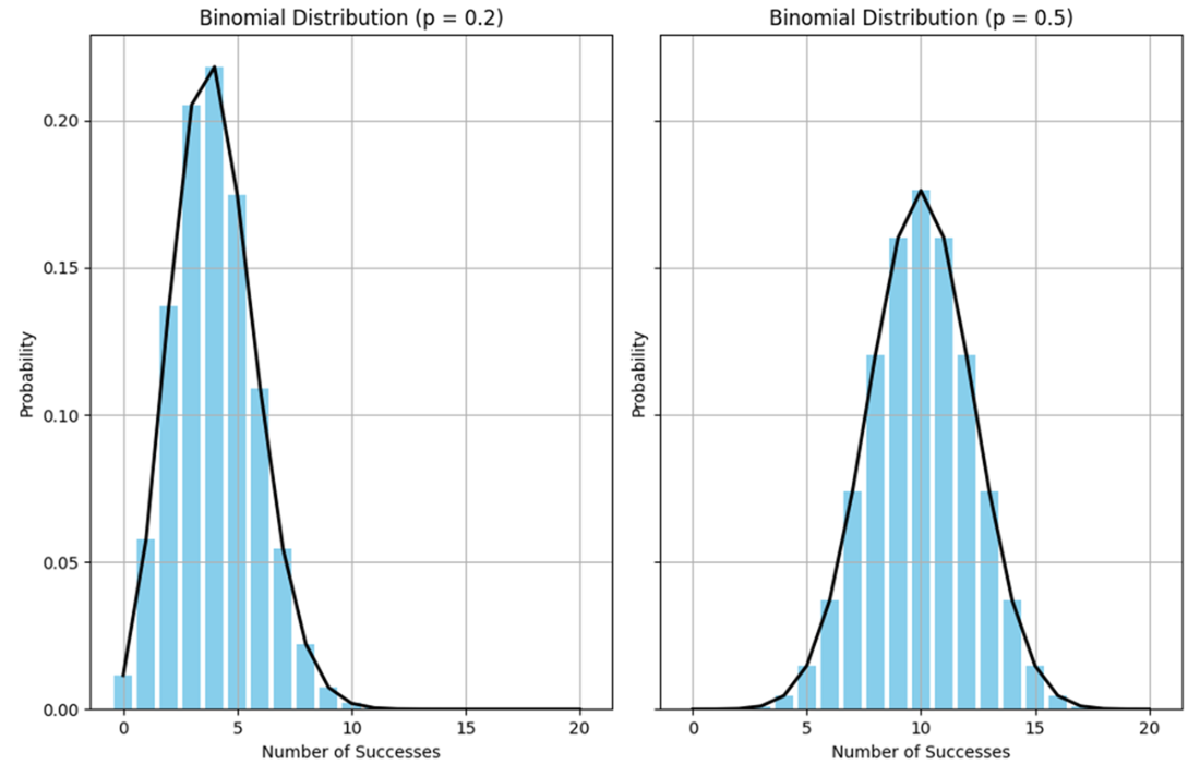
A first pair of binomial distributions where the probability of success equals 0.20 (on the left) and 0.50 (on the right), given 20 independent trials. While the distributions are binomial, the data is nonetheless distributed normally.
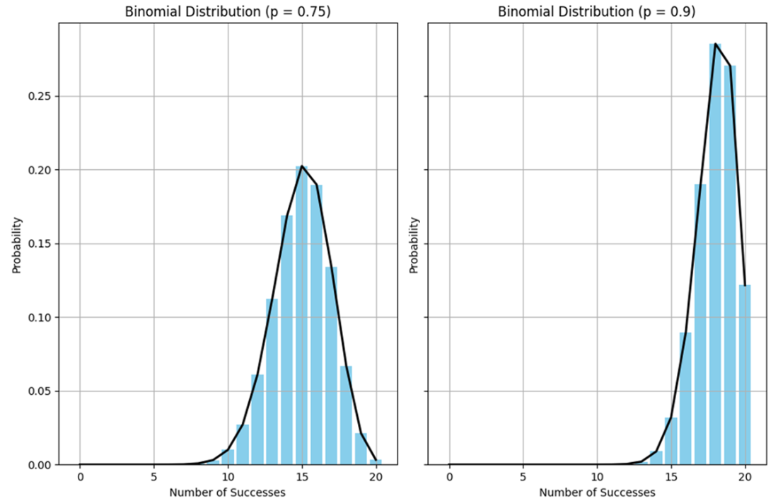
A second pair of binomial distributions where the probability of success equals 0.75 (on the left) and 0.90 (on the right), given 20 independent trials. Regardless of the probability of success, while the distribution mean shifts as a result, the binomial distributions otherwise maintain their normal distribution look.
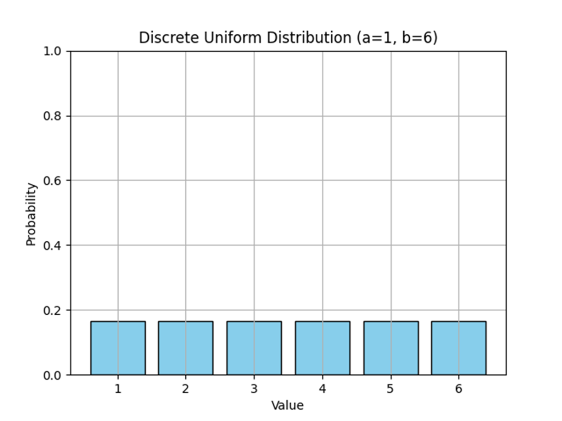
A typical discrete uniform distribution, where each discrete random variable has the same probability of occurrence. It doesn’t matter what the lower and upper bounds are; the discrete uniform distribution will always assume this rectangular shape.
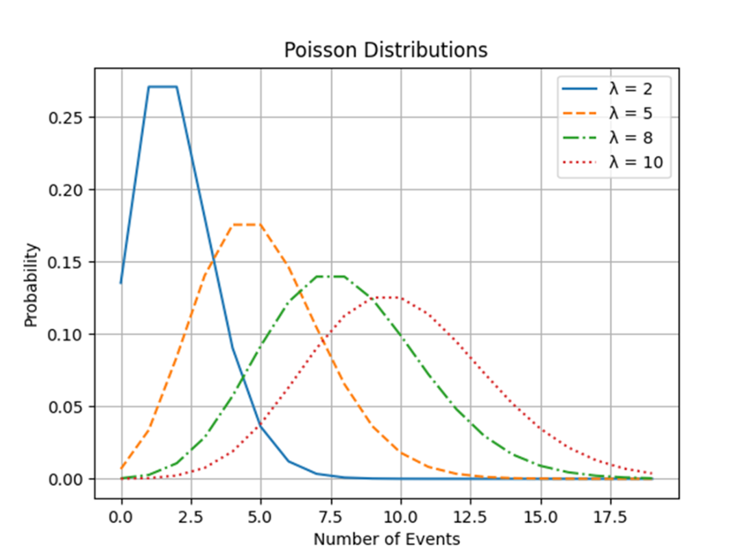
Four Poisson distributions, distinguished by their rate parameters, plotted in a single graph. As the rate parameter increases, the distribution mutates from right-skewed to normal.
Summary
- The normal distribution is a probability distribution symmetric around the mean so that, when plotted, it assumes a bell-like shape; it is defined by two parameters: the mean, which of course determines the center of the distribution, and the standard deviation, which determines the spread.
- A standard normal distribution is a special case of the normal distribution with a mean of 0 and a standard deviation of 1. The raw data has been transformed, or standardized, so that the values represent the number of standard deviations they are below or above the mean.
- The binomial distribution describes the probability of a specific number of successes in a fixed number of independent trials, where each trial has but two outcomes and the probabilities of those outcomes remain constant throughout; it is characterized by the following two parameters: the number of trials and the probability of success. Irrespective of those parameters, binomial outcomes are normally distributed.
- The discrete uniform distribution is a probability distribution where all outcomes in a finite set of values have an equal probability of occurring; it is otherwise characterized by two parameters: the number of possible outcomes and the range of values in the set.
- The Poisson distribution is a probability distribution that describes the number of events occurring within a fixed interval of time or space, given a known average rate of occurrence and assuming independence between events; it is characterized by a single parameter: the rate of occurrence.
- When computing probabilities, it’s essential to leverage a combination of various probabilities and counting rules to accurately assess the likelihood of events occurring.
- In some scenarios, it can be simpler to compute the inverse, or complement, of an event’s occurrence, thereby providing an alternative approach to understanding its probability.
- Conditional probabilities represent the likelihood of an event occurring given that another event has already occurred, thereby allowing for a deeper understanding of how events relate to each other. They are calculated by adjusting the probability of the event of interest based on additional information provided by the occurrence of another event. In other words, the sample space is reduced by decreasing the denominator and maybe the numerator as well. Which can significantly influence the dynamics of subsequent decision-making and risk assessment.
FAQ
What’s the difference between a probability density function (PDF) and an actual probability for the normal distribution?
The PDF gives relative likelihood (density) at a point; it does not equal the probability of that exact value. To get an actual probability under a normal curve, integrate the PDF over an interval (practically: use the cumulative distribution function, CDF). In practice, use a z-table or a function like norm.cdf to get areas/probabilities.What is the 68-95-99.7 (three-sigma) rule and why is it useful?
For a normal distribution, about 68% of values lie within 1 standard deviation of the mean, ~95% within 2, and ~99.7% within 3. It’s a quick way to judge how unusual a value is and to reason about variability and risk when normality is a reasonable assumption.How do I compute and use a z-score to find probabilities?
A z-score standardizes a value x by z = (x − μ) / σ. Once standardized, you can look up P(Z ≤ z) in a z-table or compute it via norm.cdf(z). To find the probability between two values, compute the two CDFs and subtract: P(a ≤ Z ≤ b) = CDF(b) − CDF(a).When should I use the binomial distribution, and what are its key properties?
Use it for a fixed number of independent trials, each with two outcomes (success/failure) and constant success probability p. The PMF is P(X = k) = C(n, k) p^k (1 − p)^(n − k). Its mean is μ = np and standard deviation is σ = √(np(1 − p)).Why do binomial histograms often look “normal”?
As the number of trials grows (and p is not extremely close to 0 or 1), the binomial distribution becomes approximately symmetric and bell-shaped. This is why binomial outcomes often resemble a normal curve in practice.What defines a discrete uniform distribution and how do I get its probabilities?
In a discrete uniform distribution over integers a through b, every value in [a, b] has equal probability 1 / (b − a + 1). Outcomes are finite, equally likely, and typically independent. Its plot is “rectangular” because all bars have the same height.What is the Poisson distribution and what does lambda (λ) represent?
The Poisson models the count of events in a fixed interval when events occur independently at a constant average rate. The rate λ is both the mean and the variance (σ² = λ). For small λ it’s right-skewed; as λ increases it becomes more symmetric and can resemble a normal distribution.How do I choose between binomial and Poisson models?
Use binomial for a fixed number of independent trials with success probability p. Use Poisson for counts over a time/space interval with an average rate λ and independence of occurrences. Poisson also approximates binomial when n is large and p is small (rare events).How do the multiplication, addition, and complement rules speed up probability problems?
- Multiplication rule: For independent events, P(A and B) = P(A)P(B).- Addition rule: For mutually exclusive events, P(A or B) = P(A) + P(B).
- Complement rule: P(A) = 1 − P(Aᶜ). Often the fastest path (e.g., “at least one” = 1 − P(none)).
 Statistics Every Programmer Needs ebook for free