2 Exploring probability and counting

This chapter surveys the essentials of probability for programmers, emphasizing why quantifying uncertainty underpins analysis and decision-making. It starts with simple, theoretical settings (coins, dice, and cards), clarifies independence and the law of large numbers, and distinguishes theoretical, empirical, and subjective probabilities. The text also shows how to express likelihoods as probabilities, percentages, and odds, and how to convert between odds and probabilities, grounding abstract ideas with small, reproducible calculations.

Next, it builds a toolkit for counting outcomes—the backbone of many probability problems. The multiplication rule handles independent, sequential or simultaneous choices; the addition rule applies to mutually exclusive options. The chapter carefully separates permutations (order matters) from combinations (order does not), and examines both with and without replacement. It introduces factorial-based formulas for nPr and nCr, quick shortcuts, and Pascal’s Triangle for combinations, then extends to combinations with replacement via a “dummy” items argument. Throughout, short Python snippets demonstrate how to compute these quantities programmatically.

Finally, the chapter formalizes random variables and contrasts continuous and discrete cases. For continuous variables, it explains the probability density function (PDF) and cumulative distribution function (CDF), highlighting properties such as non-negativity and total probability of one, with the normal distribution as a guiding example. For discrete variables, it introduces the probability mass function (PMF) and a stepwise CDF, using sums of two dice and other everyday count data to illustrate how exact probabilities accumulate. The chapter closes by teeing up the next step: studying core probability distributions that operationalize these concepts in analysis.

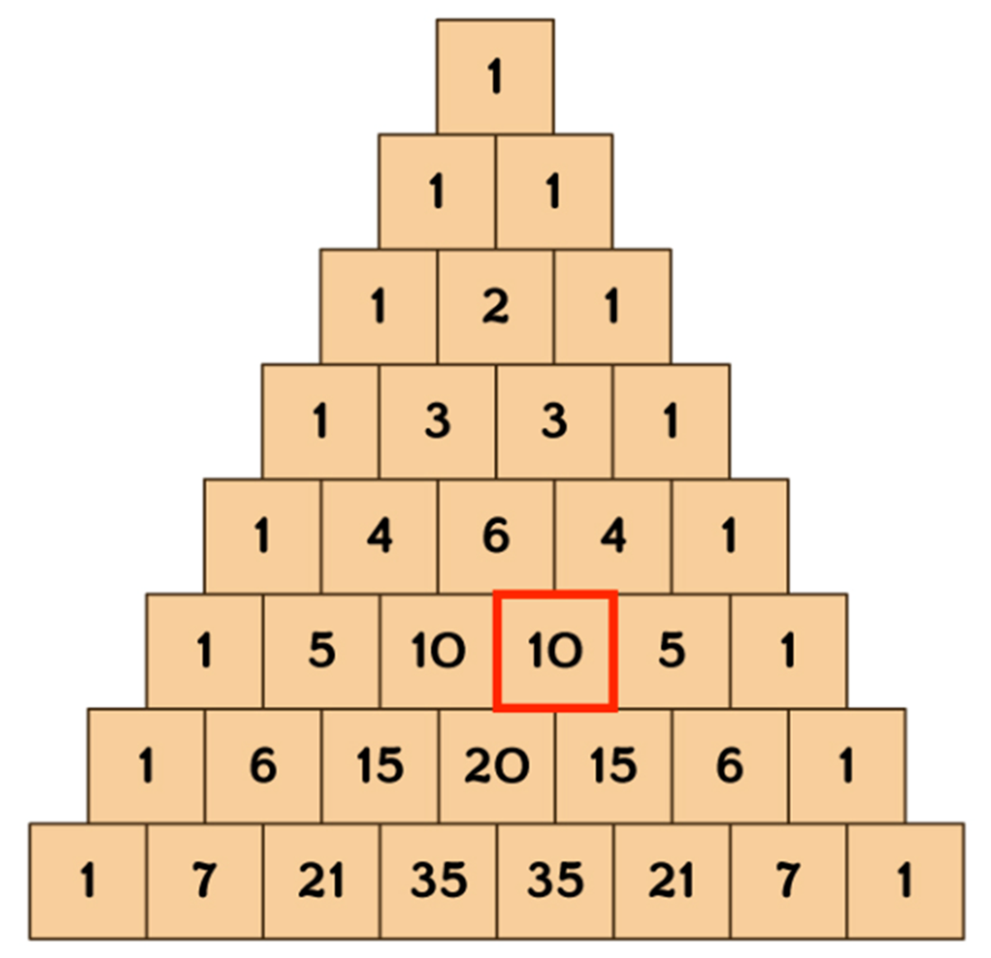
The top of Pascal’s Triangle. The triangle is constructed from the top down, where numbers are derived by adding the two numbers immediately above. It so happens that the sum of numbers for each row is twice the sum of numbers from the row above. The number of combinations without replacement can be found at the intersection of the (n + 1)th row and the (r + 1)th position in that row. When 𝑛 equals 5 (6th row down) and 𝑟 equals 3 (4th position from the left), the number of combinations without replacement equals 10.

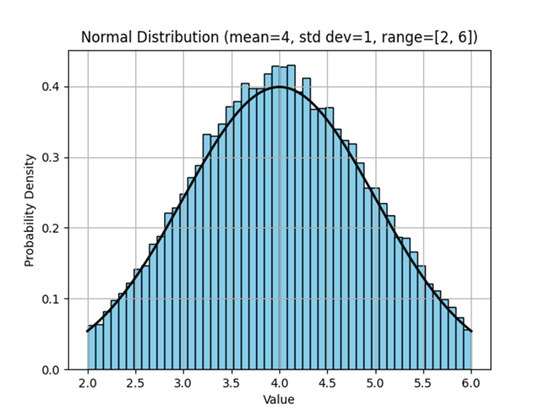
The normal distribution illustrated where the interval, or range of possible values—which runs along the x-axis—equals [2, 6]. The probability density, which runs along the y-axis, peaks at the mean, and typically tops out at approximately 0.399. The probability density for any value can therefore be estimated merely by observation. When the value equals 3.2, the probability density appears to be equal to approximately 0.30.

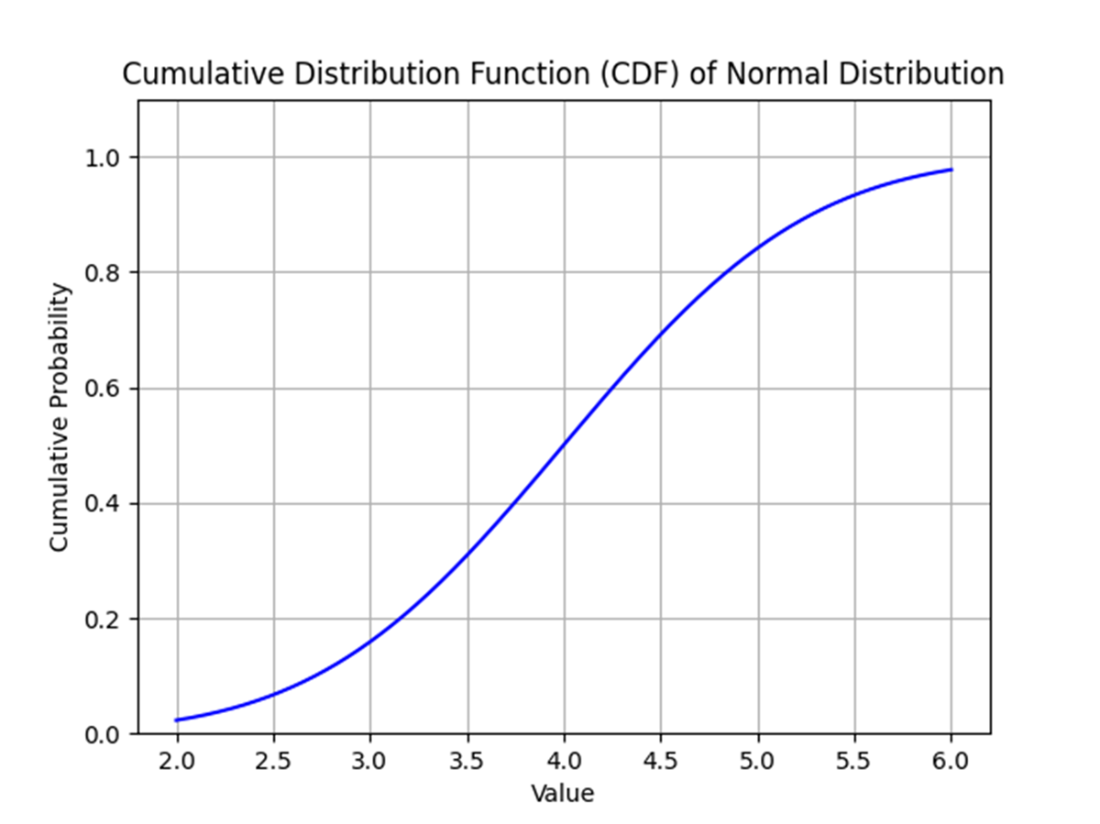
The cumulative distribution function for the normal distribution when the lower and upper bounds equal 2 and 6, respectively; the mean equals 4, and the standard deviation equals 1. The shape of the cumulative distribution function will vary depending on the probability density function being modeled; regardless, it will always start at 0 and top out at 1.

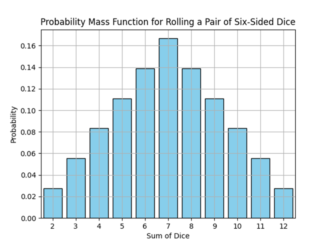
The probability mass function for rolling a pair of six-sided dice, where the discrete random variable and its possible values, which are equal to the whole numbers between 2 and 12, are plotted along the x-axis, while their respected probabilities of occurrence are plotted along the y-axis. The y-axis represents their actual probabilities and not their relative likelihood of occurrence. All probabilities are equal to or greater than zero.

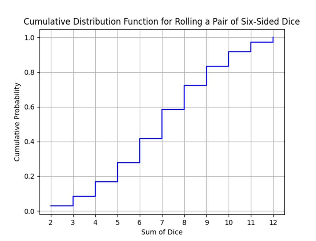
The cumulative distribution function for rolling a pair of six-sided dice. The shape of the distribution resembles a two-dimensional flight of stairs, in which the horizontal line segments represent consecutive values for 𝑥, while the vertical lines represent their respective probabilities.

• Theoretical probabilities are equal to the number of successes divided by the total number of possible outcomes.
• Empirical probabilities are derived from trials or real-world observations; such probabilities are equal to the number of successes observed (however a “success” might be defined) divided by the number of observations made.
• The multiplication rule states that the probability of two or more events occurring is equal to the product of their individual probabilities. This rule applies to independent events that occur simultaneously or sequentially.
• The addition rule, meanwhile, states that the probability of two or more mutually exclusive events occurring is equal to the sum of their individual probabilities. This rule applies when the events cannot occur simultaneously.
• Combinations and permutations are not the same. A combination refers to the selection of items where the order does not matter, while a permutation involves arrangements where the order means everything. Combinations apply to scenarios like choosing a group of students to sit on a committee, whereas permutations apply to situations like arranging a sequence of numbers or letters.
• A permutation with replacement is a method of arranging items from a set where each item can be chosen multiple times for each position in the arrangement. This allows for the repetition of items in the arrangement, resulting in a larger number of possible permutations compared to permutations without replacement.
• A permutation without replacement, on the other hand, is a method of arranging items from a set where each item can be chosen only once for each position in the arrangement. This ensures that each item appears no more than once in the final arrangement, leading to fewer permutations compared to permutations with replacement.
• A combination without replacement is a selection of items from a set where each item can be selected no more than once, and the order of selection does not matter. This ensures that each item is selected maybe once for the combination, leading to a unique subset of items from the original set.
• Conversely, a combination with replacement is a selection of items from a set where each item can be chosen multiple times, and the order of selection does not matter. This allows for the repetition of items in the combination, resulting in a larger number of possible combinations compared to combinations without replacement.
• A continuous random variable is a type of random variable that can take on any value within a certain range, oftentimes representing measurements or quantities that can be infinitely subdivided.
• While a discrete random variable is a type of random variable that can only take on a countable number of distinct values, oftentimes representing outcomes of experiments or events that result in a finite or countably infinite set of possible outcomes. Unlike continuous random variables, which can assume any value within a range, discrete random variables have specific and separate values with no intermediate possibilities.

FAQ