6 Tabular Reinforcement Learning

This chapter positions temporal-difference (TD) learning as the load‑bearing wall of reinforcement learning and pairs it with generalized policy iteration as the field’s core. It traces the path from Markov chains and Bellman’s dynamic programming to model‑free TD methods that learn directly from experience, emphasizing online, incremental updates driven by prediction error. The TD error—the gap between what happened and what was expected—serves as a practical, biologically plausible learning signal that lets agents improve without full knowledge of transition dynamics, aligning closely with how businesses and organisms adapt under uncertainty.

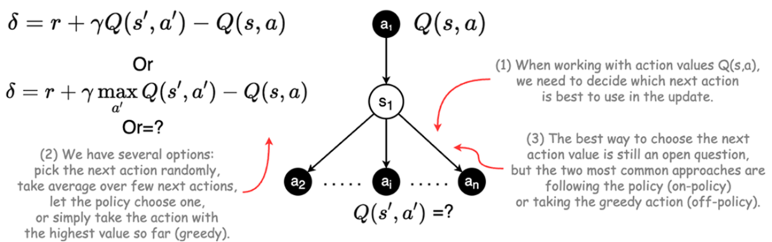
Building on this foundation, the chapter explains how sampling replaces explicit expectations and why action values Q(s,a) become central in model‑free control. It clarifies exploration–exploitation and the bootstrap nature of TD, then contrasts on‑policy and off‑policy learning through SARSA and Q‑learning. SARSA updates from the action the agent actually takes, yielding conservative, risk‑aware behavior; Q‑learning learns toward the greedy target regardless of behavior, often converging faster but with optimistic bias. In tabular settings, knowledge is stored in lookup tables (Q‑tables), making learning transparent and direct. A simple restaurant scheduling example demonstrates TD’s convergence to dynamic‑programming optima purely from experience.

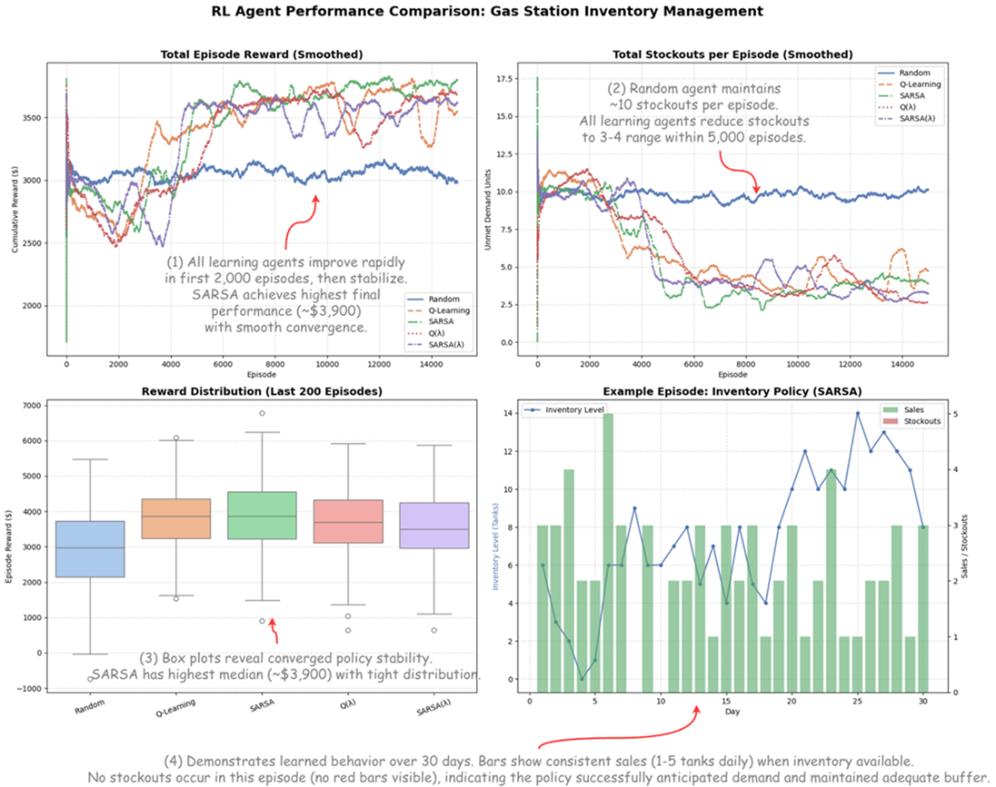
The chapter extends one‑step TD to multi‑step credit assignment with TD(λ) and eligibility traces, showing how λ trades bias for variance and how traces efficiently propagate credit backward in time. It distinguishes accumulating versus replacing traces, and explains on‑policy SARSA(λ) versus Watkins’s off‑policy Q(λ), which resets traces after non‑greedy actions to preserve off‑policy correctness. A realistic gas‑station inventory case study ties everything together: tabular agents learn profitable, robust ordering policies under stochastic demand and delivery delays, revealing practical trade‑offs—e.g., SARSA’s stability and realistic risk handling, Q‑learning’s efficiency and lower stockouts, and situations where added algorithmic complexity (eligibility traces) may not outperform simpler baselines.

Like cooking, we use feedback from error to update parameters step by step.

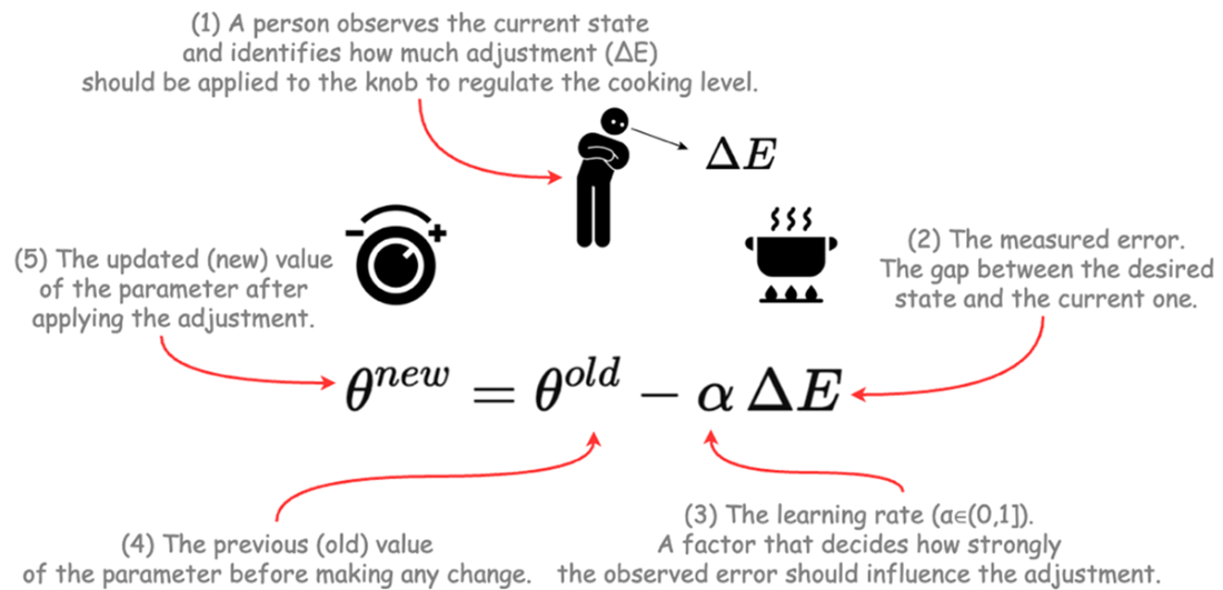
The formula shows how each update moves the old value toward a better one.

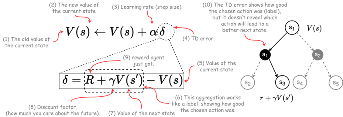
Convergence behavior of Temporal difference learning algorithm.

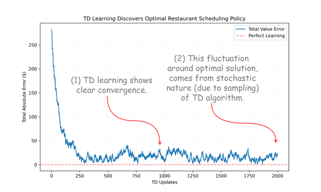
illustration of problem of aligning within the TD framework

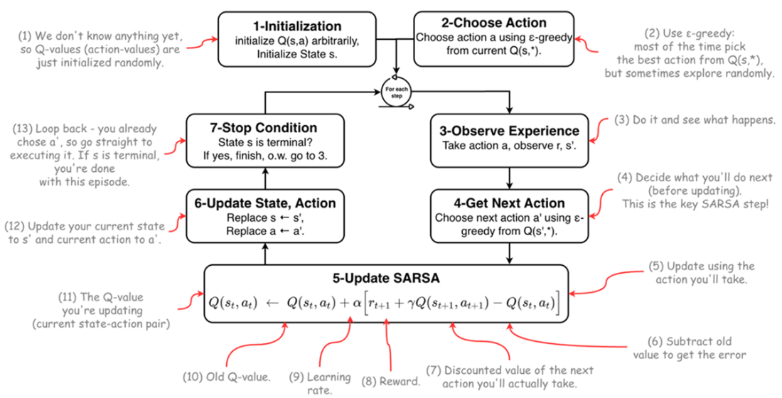
SARSA Algorithm Flowchart.

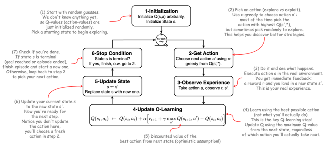
Q-learning Algorithm Flowchart.

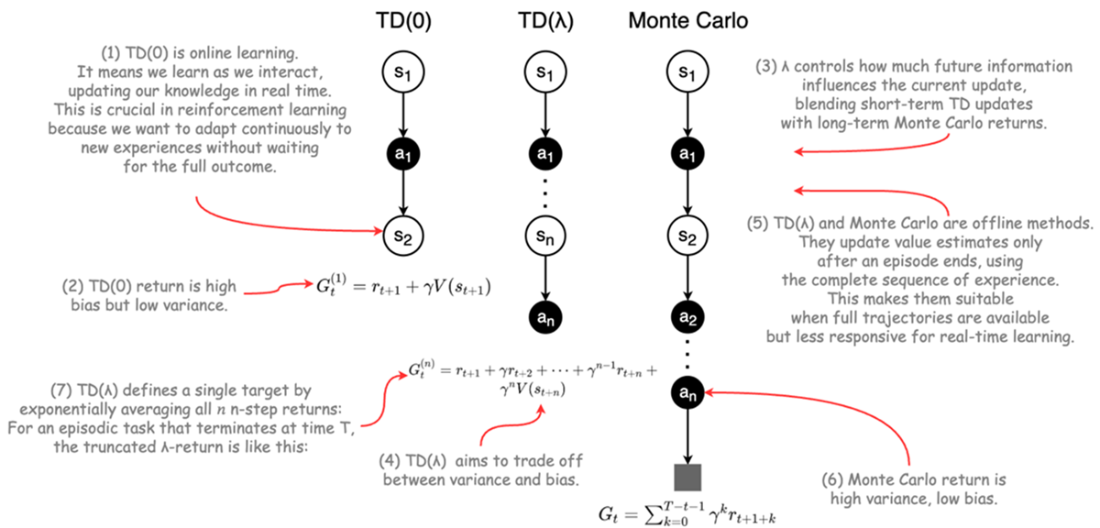
Comparison of TD(0), Monte Carlo and TD(λ) methods.

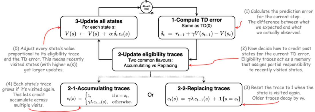
Update mechanism of temporal difference learning with eligibility traces.

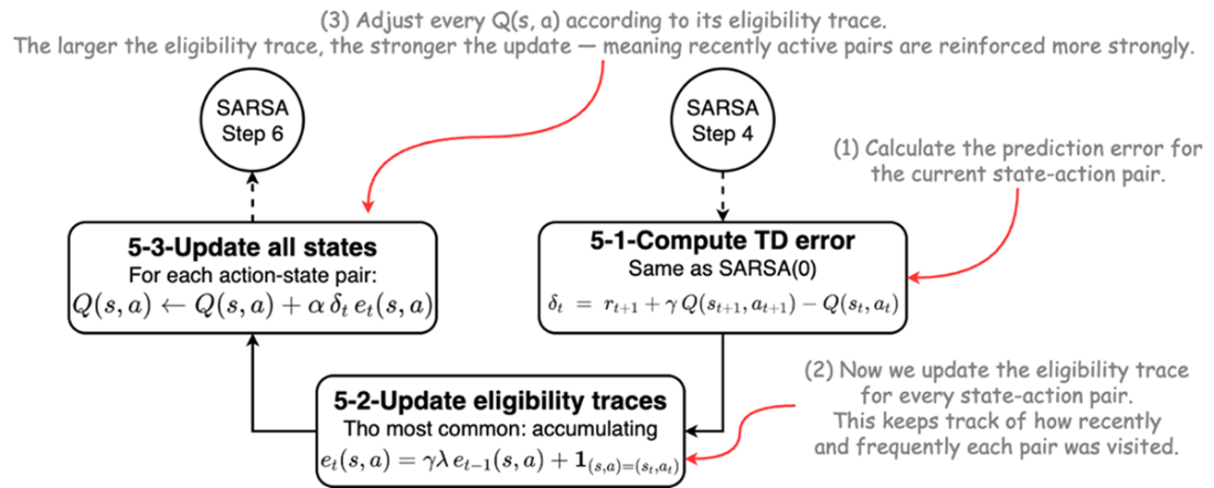
integrating eligibility trace in SARSA framework: SARSA(λ).

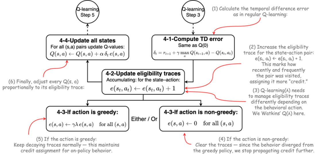
Integrating eligibility traces with Q-learning using Watkins's Q(λ) method.

Tabular Reinforcement Learning Curves and Performance Analysis.

• In model-based learning, the agent has access to the full dynamics of the environment—the transition probabilities P(s'|s,a) and reward function R(s,a). Dynamic Programming is a model-based approach.
• In model-free learning, the agent does not know these dynamics and must learn directly from experience tuples (s, a, r, s') gathered through trial and error. Temporal difference learning, Q-learning, and SARSA are all model-free.
• In offline learning, the agent is trained on a fixed, pre-collected batch of data and does not learn during interaction.
• In online learning, the agent updates its knowledge continuously during interaction with the environment, learning step-by-step as new experience arrives. All the temporal difference methods discussed in this chapter are online learners.
• In on-policy learning, the agent learns to improve the same policy it is using to make decisions. It learns from its own "lived experience." SARSA is on-policy.
• In off-policy learning, the agent can learn about a different policy (the target policy, typically the optimal one) than the one it is using to generate behavior (the behavior policy, typically an exploratory one). Q-learning is off-policy.
• Temporal-Difference learning is one of the two pillars of reinforcement learning, enabling agents to learn from raw experience without a model of the environment.
• The core idea of temporal difference learning is to update your predictions based on the error between your current guess and a slightly better guess one step into the future.
• This process of updating estimates using other estimates is called bootstrapping, and it allows learning to happen online, after every single step.
• The TD error (δ) is the learning signal, quantifying the "surprise" or difference between what you expected and what you observed.
• Temporal difference learning is the bridge between Dynamic Programming (which needs a full model) and Monte Carlo methods (which must wait for an episode to end).
• For an agent to make decisions in a model-free world, it must learn action values (Q(s,a)), not just state values (V(s)).
• Tabular methods represent the value function as a lookup table or spreadsheet, with a distinct entry for every state-action pair.
• Q-learning is the quintessential off-policy algorithm; it learns about the optimal greedy policy while behaving according to a different, more exploratory policy.
• Because Q-learning uses the max Q-value for its update, it is considered optimistic and often converges faster to the optimal policy.
• SARSA is the quintessential on-policy algorithm; it learns about the same policy it is using to make decisions, including all its exploratory actions.
• Because SARSA's updates use the Q-value of the actual next action taken, it is considered more realistic or conservative, learning a policy that is robust in the face of its own exploration.
• The credit assignment problem asks how to distribute credit for a reward among the many actions that may have led to it, especially when rewards are delayed.
• Eligibility traces (TD(λ)) are the solution, creating a short-term memory that allows the TD error to be propagated backward to all recently visited state-action pairs.
• The λ parameter controls how far back credit is assigned, providing a tuneable spectrum between one-step TD (λ=0) and Monte Carlo (λ=1).
• SARSA(λ) is a highly effective on-policy algorithm that combines the stability of SARSA with the learning speed of eligibility traces.
• Watkins's Q(λ) adapts traces for off-policy learning by resetting the traces to zero whenever a non-greedy (exploratory) action is taken.

FAQ