4 Applying Post-Training Quantization and Calibration

This chapter shows how to ship accurate, fast post-training quantized models by combining sound decision-making, careful calibration, and disciplined validation. It first clarifies when post-training quantization (PTQ) is sufficient and when to escalate to quantization-aware training (QAT). Four factors reliably predict PTQ success: model architecture (and its sensitivity to perturbations), target bit-width (with a steep drop in robustness below INT8), model size/redundancy (capacity to absorb noise), and acceptable accuracy loss (a business threshold). The key guidance is pragmatic: INT8 PTQ with per-channel weights typically works out of the box; INT4 demands group-wise schemes; and attention-heavy transformers are the hard cases that may need advanced calibration or mixed precision before considering QAT.

Calibration is framed as discovering activation ranges your model will truly see in production. The central risk is distribution mismatch: if calibration data under-represents difficult conditions or key user segments, ranges will be misestimated—either wasting precision or clipping frequently. “Representative” therefore means covering activation space, not just mirroring average inputs. In practice, a compact but diverse set (often 128–512 samples) that stresses extremes—lighting and contrast in vision, and prompt length, task/linguistic variety, and structured content in LLMs—beats large but homogeneous collections. A repeatable workflow closes the loop: deploy an initial full-precision model with activation instrumentation, compare per-layer production maxima to calibration coverage, fill gaps, and revalidate periodically as traffic evolves.

The chapter then details range estimation methods and a simple diagnostic to choose among them. Absolute maximum avoids clipping but can squander precision on outliers; percentile clipping trades tiny, bounded clipping for better resolution; MSE-optimal directly minimizes reconstruction error and is a strong default for transformer activations; KL/entropy can fail on heavy-tailed distributions. Computing an outlier ratio (max/99th percentile) guides selection: low ratios favor absmax, mid/high ratios favor high-percentile or MSE-optimal. Finally, a validation protocol ties it together: measure an FP32 baseline, quantize with multiple calibration methods, track quantization error and task metrics, aim for sub‑1% accuracy loss, verify the expected 4× size reduction for INT8, and investigate misses via improved calibration, per-channel/group quantization, or mixed precision. True latency gains require INT8-capable runtimes; once accuracy and coverage are proven, deployment becomes an engineering exercise rather than a research project.

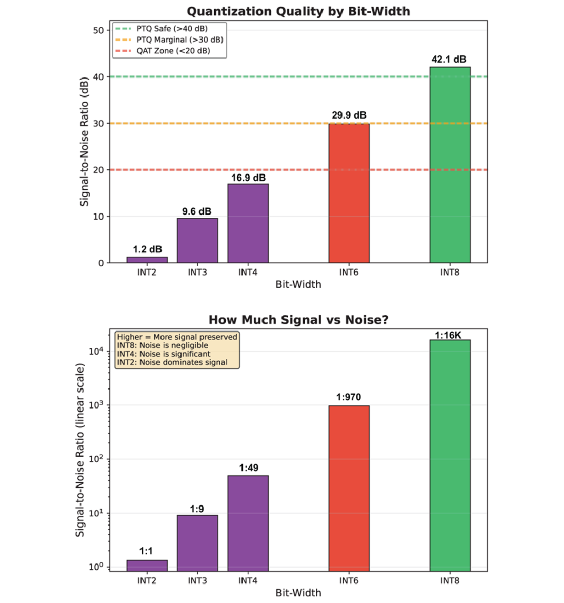
Left: Signal-to-Noise ratio by bit-width with PTQ viability zones. Right: Signal-to-noise ratio as intuitive ratios

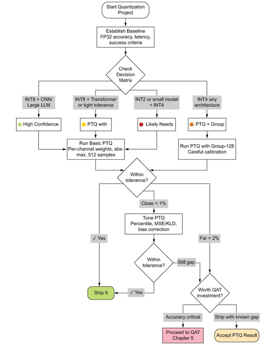
PTQ decision framework flowchart. Starting from the target bit-width at the top, the reader follows branching decisions through model architecture checks, calibration method selection, and accuracy validation gates. Each terminal node recommends either shipping the PTQ result or escalating to QAT.

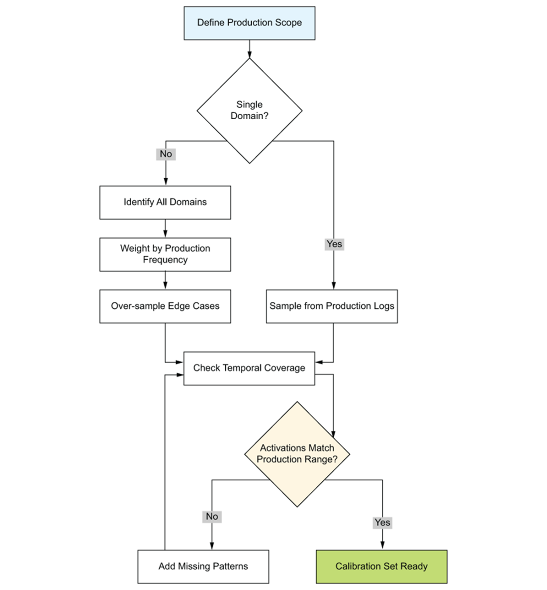
Workflow for preparing a calibration set. The process flows from top to bottom: source production data from logs or traffic samples, apply stratified sampling to cover user segments and edge cases, validate distribution coverage against known activation patterns, and iterate if coverage gaps are found. Each stage includes a quality gate that prevents poorly representative data from reaching calibration.

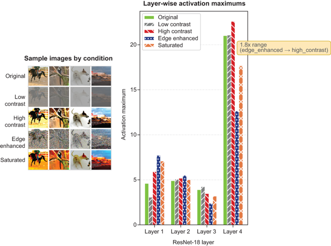
Left: Sample images under four conditions (original, low-light, high-contrast, noisy) showing the visual transformations applied to STL-10 images. Right: Layer-wise activation maximums through ResNet-18, where each line corresponds to one condition. Notice how low-light images produce consistently lower activation ranges while high-contrast images push activation maximums higher in deeper layers—calibrating on only one condition would systematically mis-estimate the ranges encountered in production.

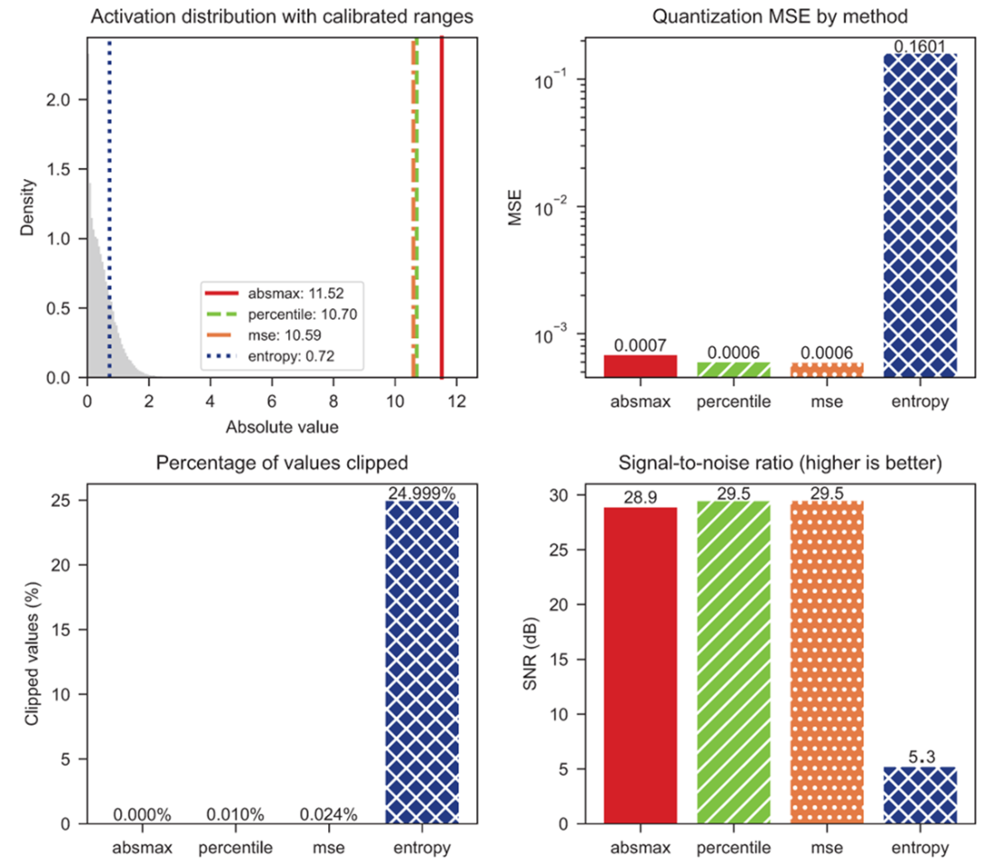
Comparison of range estimation methods on BERT-base layer 6 activations

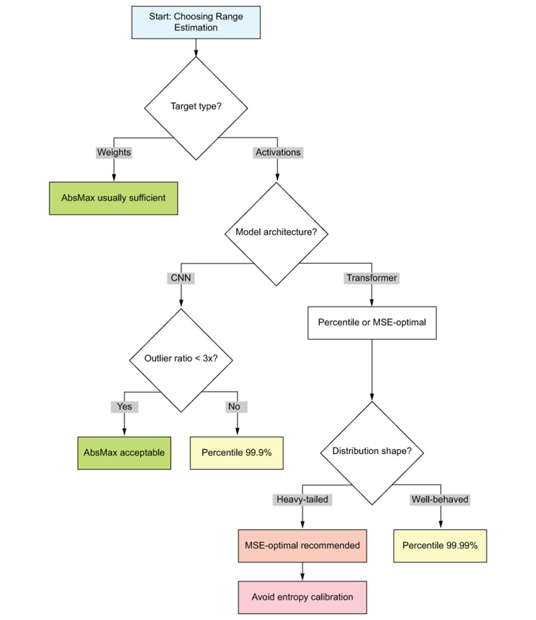
Decision framework for range estimation method selection. Start by computing the outlier ratio (max / 99th percentile) on your calibration data. If the ratio is below 2×, activations are well-behaved and absolute maximum (absmax) is sufficient. Between 2–10×, percentile clipping at 99.99% provides a safe default. Above 10×, use MSE-optimal calibration to automatically find the best clipping threshold. The framework routes you to the simplest method that handles your distribution shape.

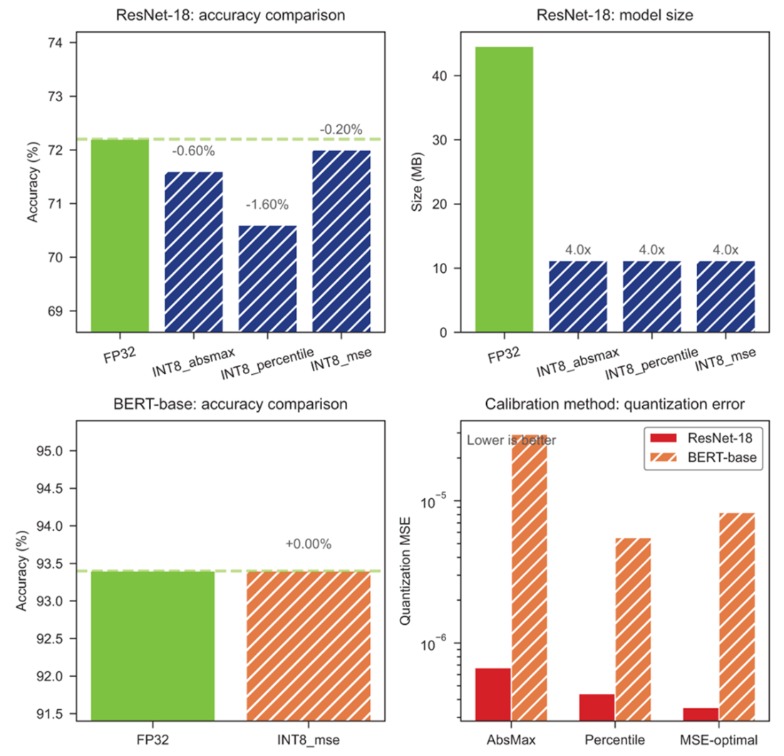
MSE calibration preserves accuracy best (top-left); MSE-optimal achieves lowest quantization error across architectures (bottom-right)

• PTQ works best for INT8 quantization of CNNs and BERT-scale transformers with smooth weight distributions—it delivers 4× size reduction with minimal accuracy loss and zero retraining.
• Calibration data determines quantization ranges, so your calibration set must match production data distribution. A few hundred representative samples usually suffice, covering edge cases and deployment scenarios.
• MSE-optimal range estimation delivered the best accuracy in our experiments (ResNet: -0.20%, BERT: 0.00% loss), though absmax works for clean distributions and percentile helps with sparse outliers.
• Size reduction is guaranteed (4× for INT8 is arithmetic), but accuracy preservation depends on calibration quality—always validate against FP32 baseline before deployment.
• Latency improvement requires runtime support (PyTorch quantization backends, TensorRT, or ONNX Runtime)—storing INT8 weights alone won't speed up inference without proper execution backends.
• When PTQ fails to meet accuracy targets, the path forward is Quantization-Aware Training (Chapter 5) for strict requirements or specialized LLM techniques (Chapter 7) for sub-8-bit precision.

FAQ