3 Blind Search Algorithms

This chapter introduces blind (uninformed) search within deterministic algorithms and grounds it in graph fundamentals. It describes graphs as collections of vertices and edges that can be directed or undirected, multigraphs with parallel edges, acyclic structures, hypergraphs that connect many nodes at once, and weighted networks where edge costs matter. The text emphasizes how these representations model real systems—social networks, telecommunications, and especially road networks—and shows how common tooling can construct and explore such graphs. With this foundation, the chapter motivates blind search as a practical, repeatable approach for exploring state spaces and finding paths in well-defined problems such as sliding-tile puzzles, family trees, social connections, mazes, and city routing tasks.

Two traversal methods anchor the discussion: Breadth-First Search (BFS) and Depth-First Search (DFS). BFS expands level by level using a FIFO queue, guarantees finding a solution if one exists in a finite graph, and is well suited to shallow goals but can be memory intensive (time and space grow rapidly with branching factor and depth). DFS descends along a path using a LIFO stack, backtracks at dead ends, and is memory efficient but can wander deep without finding nearby solutions; a depth limit can mitigate this. Through examples like the 8‑puzzle and grid-based path planning, the chapter contrasts their behaviors and introduces Big‑O analysis to reason about scalability, highlighting trade-offs between time, space, and problem structure when selecting a traversal strategy.

For optimal routing on weighted graphs, the chapter presents Dijkstra’s algorithm, Uniform-Cost Search (UCS), and Bidirectional Dijkstra. Dijkstra computes shortest paths with non‑negative edge costs via a priority queue; UCS is a practical variant that grows the frontier incrementally and reduces overhead, behaving like BFS when all edges have equal cost; bidirectional search runs forward from the source and backward from the goal to cut the search space dramatically. A campus routing case study shows that these methods produce identical optimal routes while differing in time and memory usage. The chapter also notes practical details for real maps—choosing the lightest among parallel edges and ignoring self‑loops to avoid path reconstruction issues. It concludes that BFS/DFS can find feasible (not necessarily optimal) routes quickly, whereas Dijkstra/UCS/Bidirectional Dijkstra yield provably shortest paths, and previews how informed search will leverage domain knowledge to improve efficiency further.

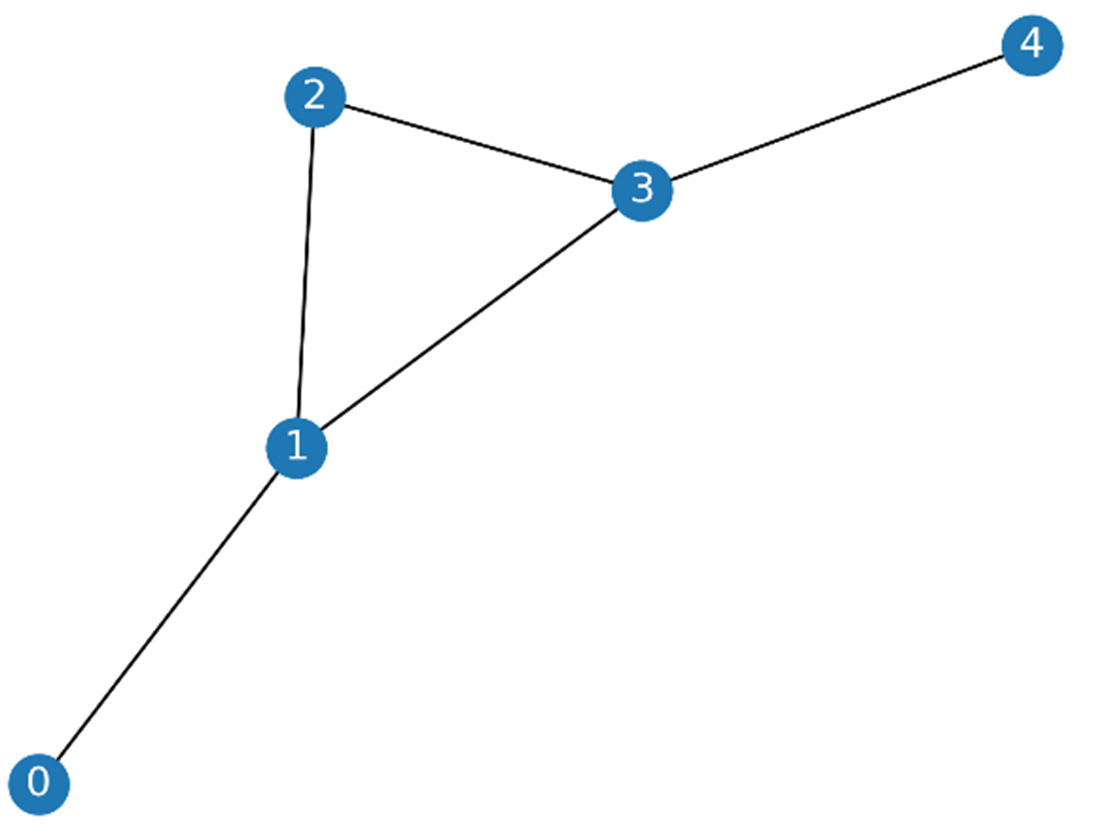
Undirected graph.

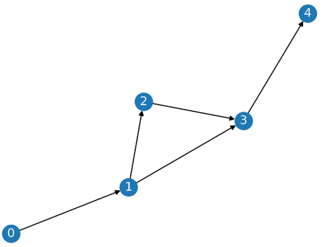
A directed graph.

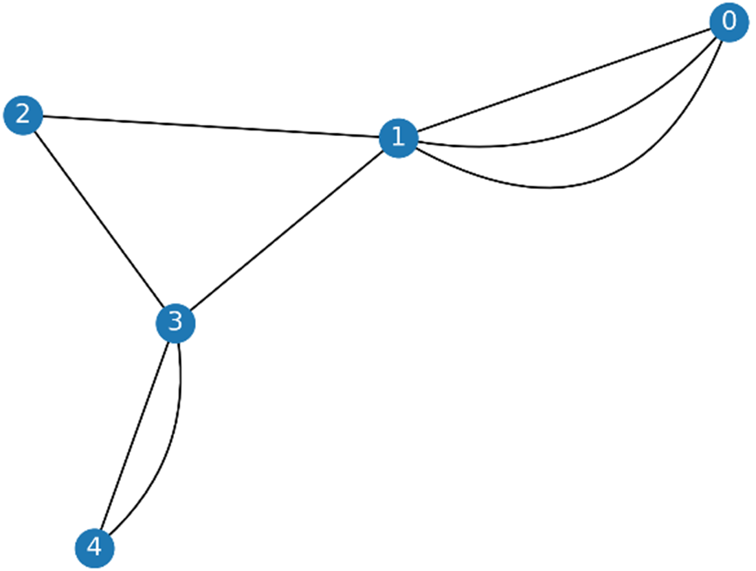
Example of a multi-graph. Notice the three parallel edges connecting nodes 0 and 1, as well as the two edges connecting nodes 3 and 4.

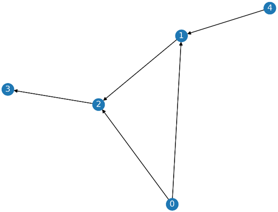
An acyclic graph. There is no path that cycles back to any starting node.

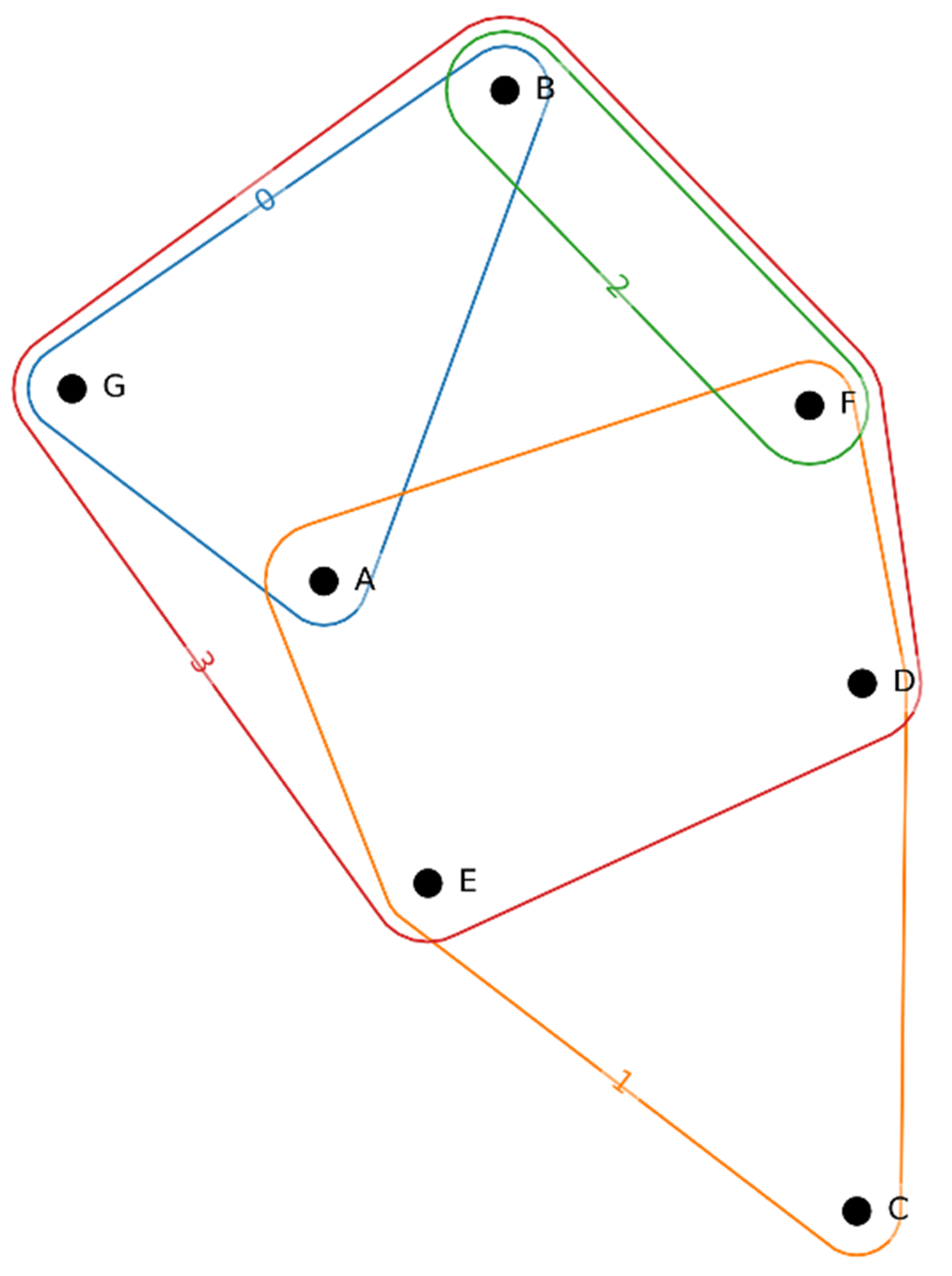
An example of a hypergraph. Hyperedges can connect more than two nodes, such as hyperedge 0, which links nodes A, B, and G.

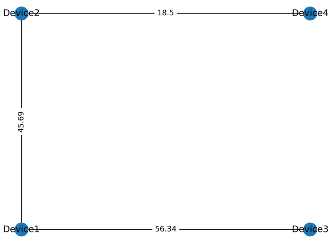
Example of a weighted graph.

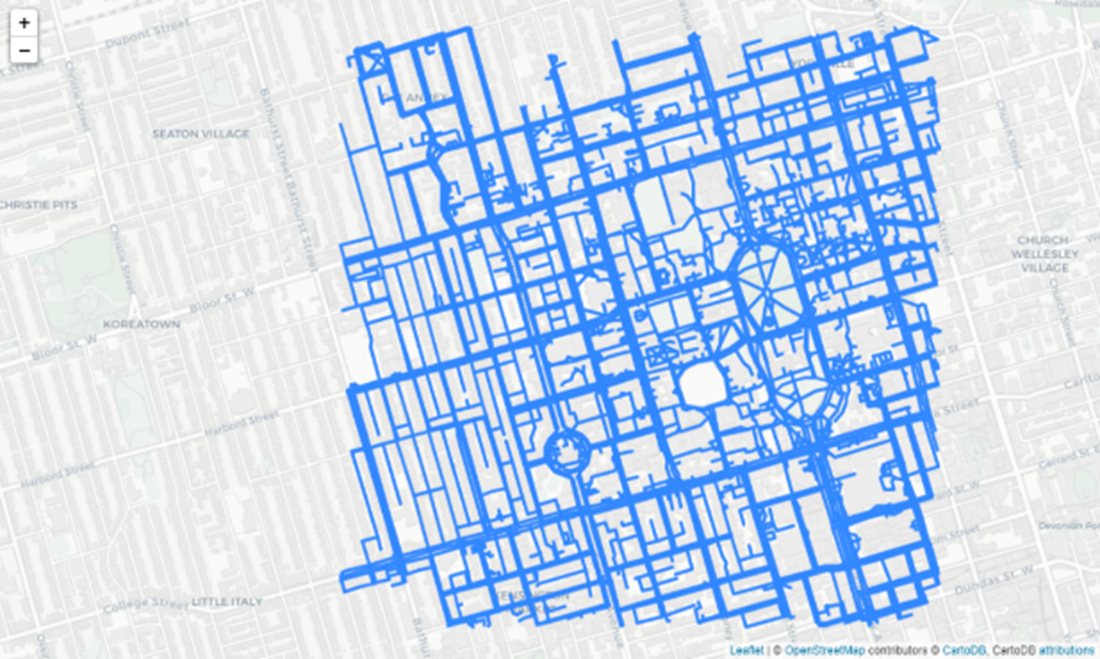
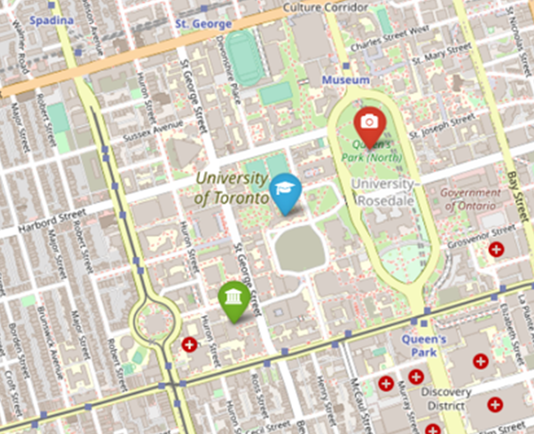
St. George Campus - University of Toronto

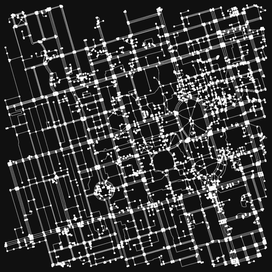
Road network around St. George Campus - University of Toronto

Visualizing points of interest using folium markers

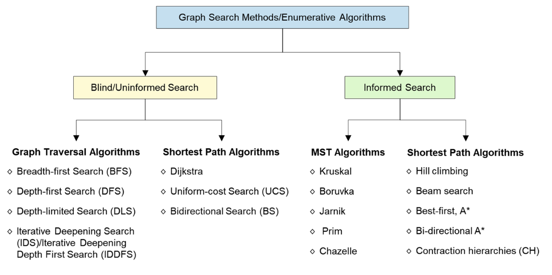
Graph Search Methods.

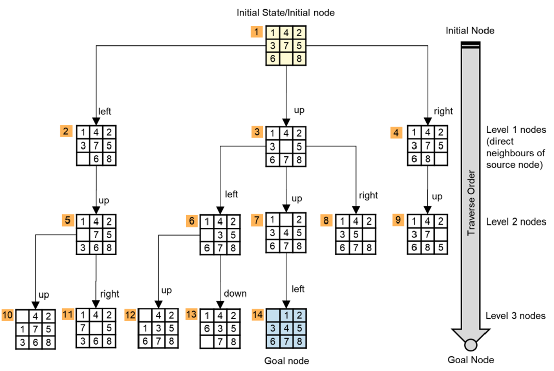
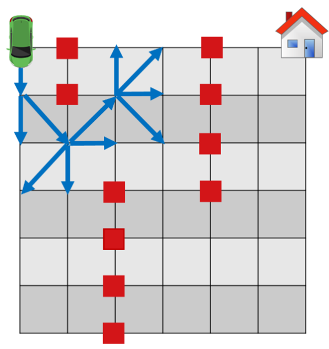
Using BFS to solve 8-puzzle problem

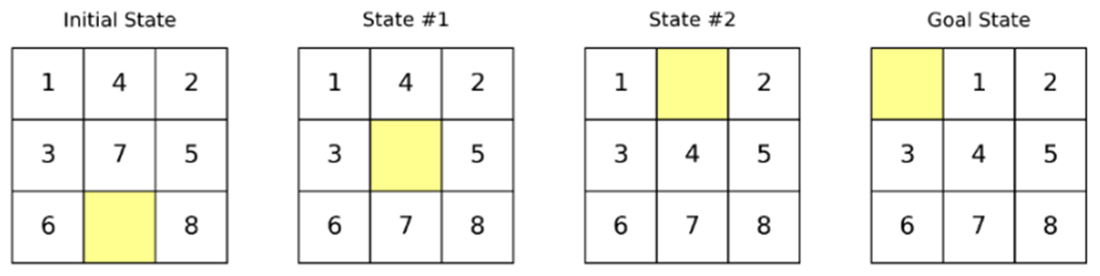
Step-by-step BFS solution using Python. BFS searches for a solution but does not consider optimality.

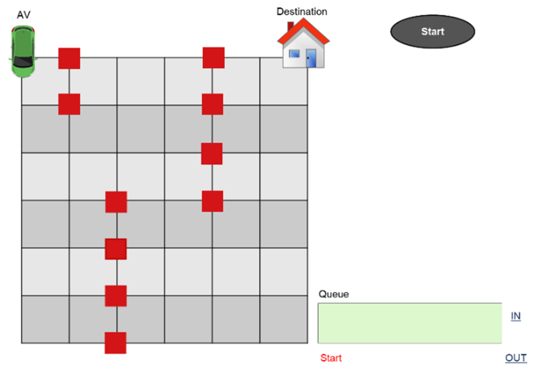
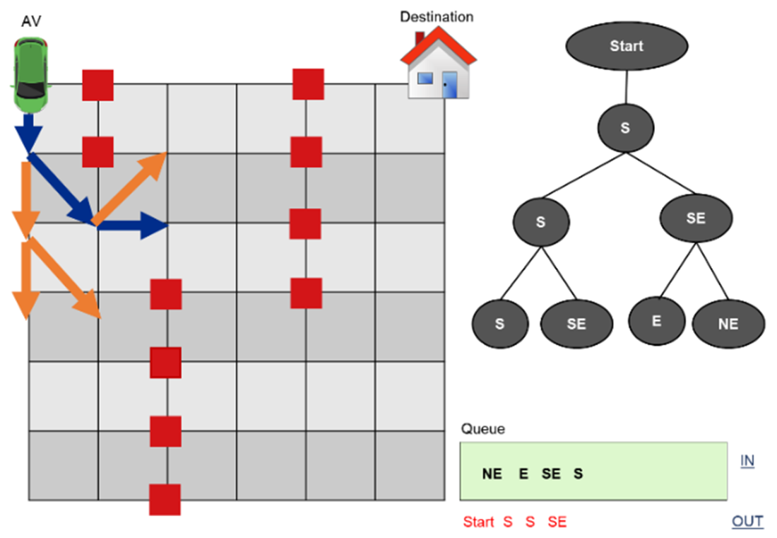
Solving path planning problem using BFS – Step 1

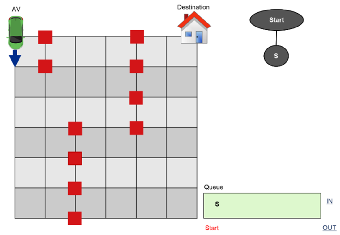
Solving path planning problem using BFS – Step 2

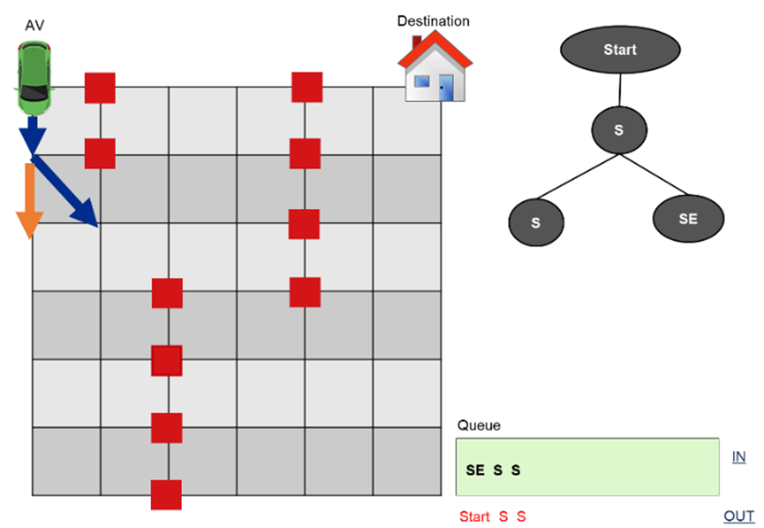
Solving path planning problem using BFS – Step 3

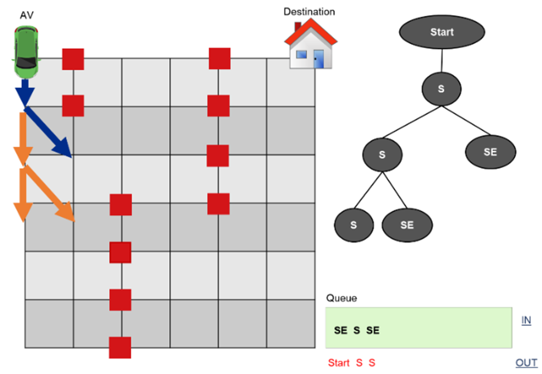
Solving path planning problem using BFS – Step 4

Solving path planning problem using BFS – Step 5

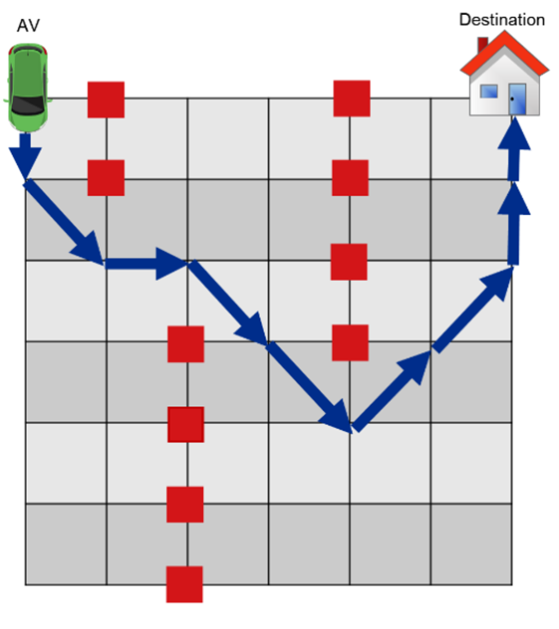
Solving path planning problem using BFS – Final route

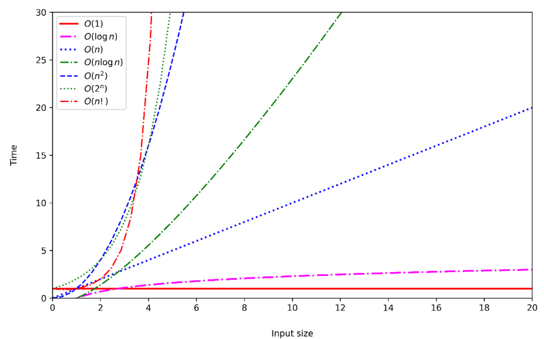
Examples of big O notations

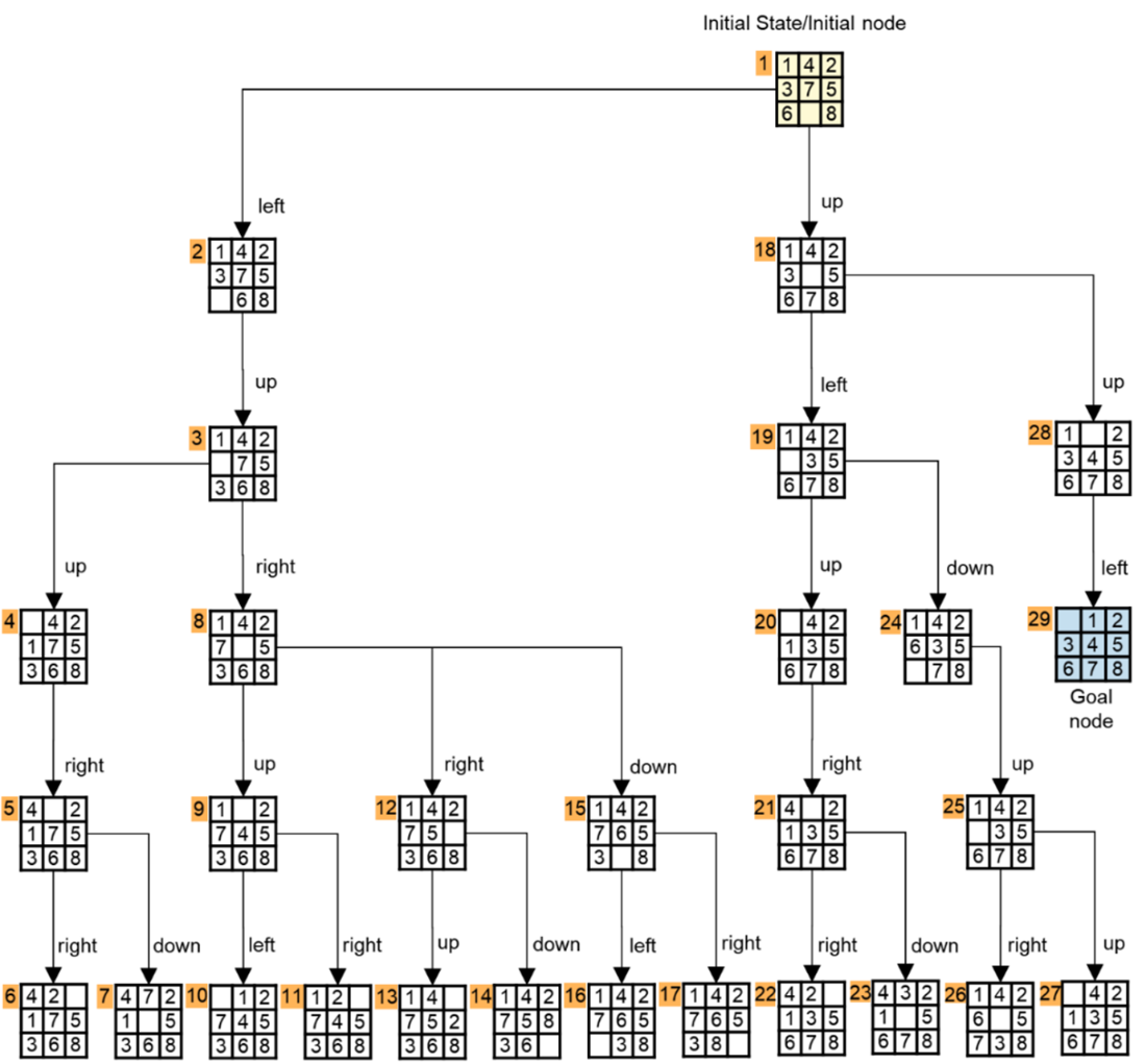
Using DFS to solve the 8-puzzle problem

Solving path planning problem using DFS – Step 1

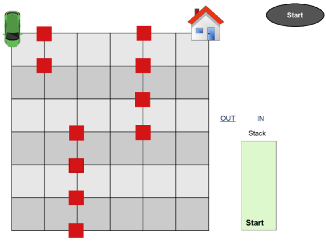
Solving path planning problem using DFS – Step 2

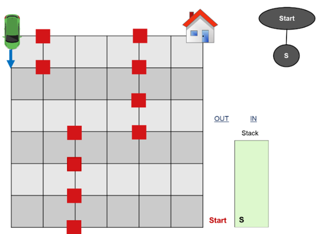
Solving path planning problem using DFS – Step 3

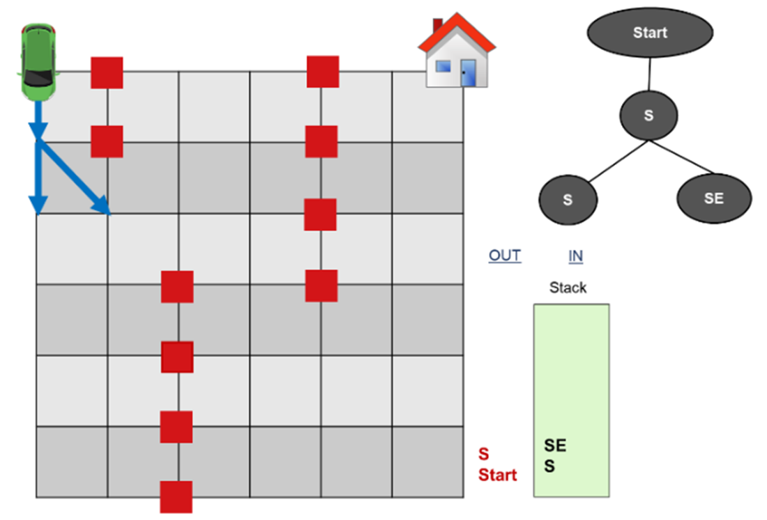
Solving path planning problem using DFS – Step 4

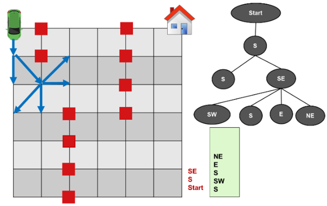
Solving path planning problem using DFS

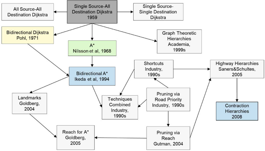
Dijkstra’s algorithm and its variants

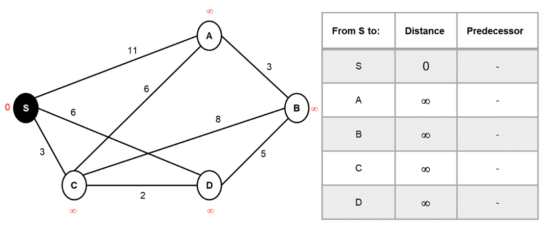
Finding shortest path using Dijkstra’s algorithm – Step 0

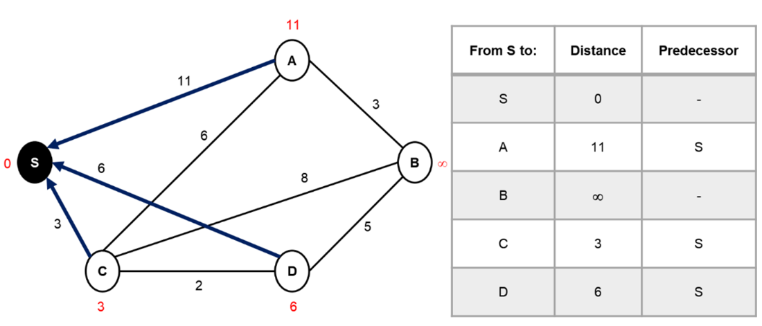
Finding shortest path using Dijkstra’s algorithm – Step 1

Finding shortest path using Dijkstra’s algorithm – Step 2

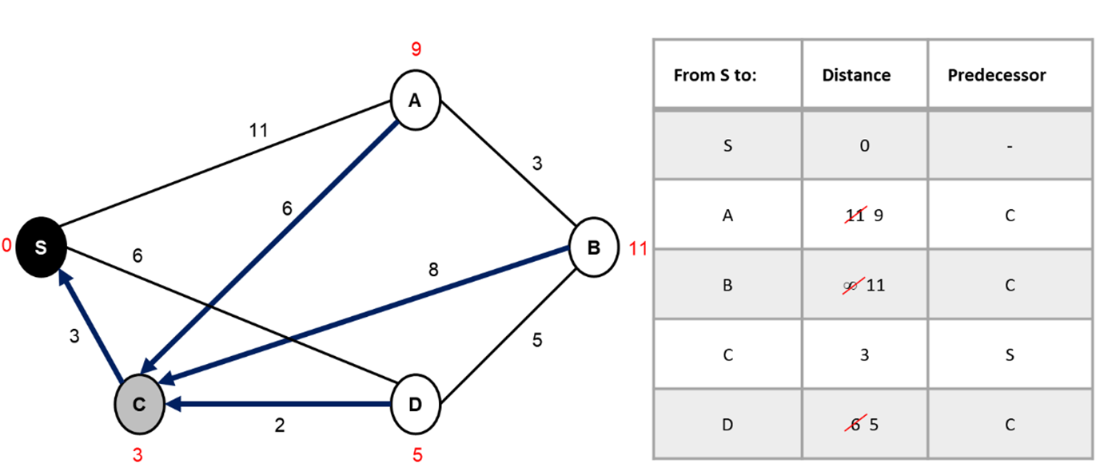
Finding shortest path using Dijkstra’s algorithm – Step 3

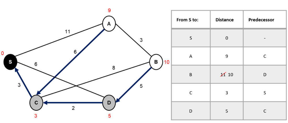
Finding shortest path using Dijkstra’s algorithm – Step 4

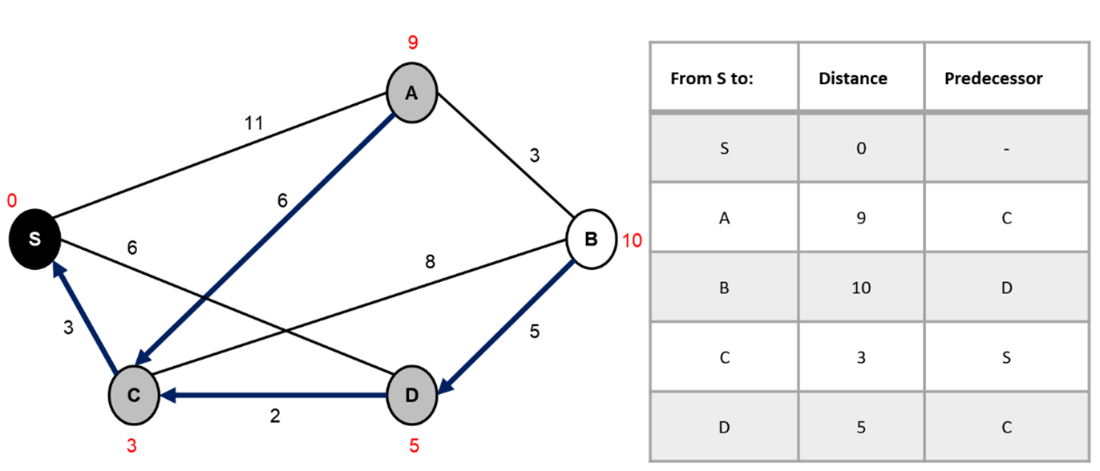
Finding shortest path using Dijkstra’s algorithm – Step 5

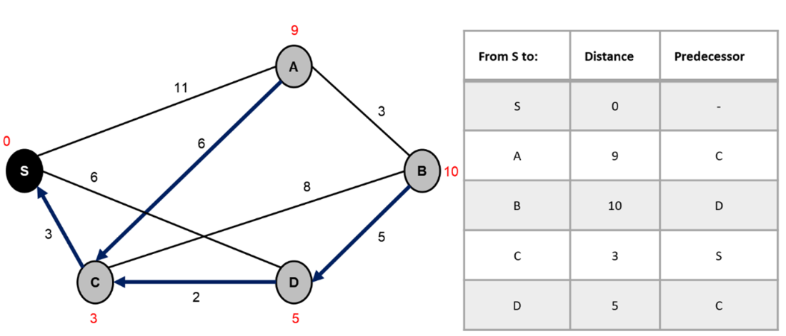
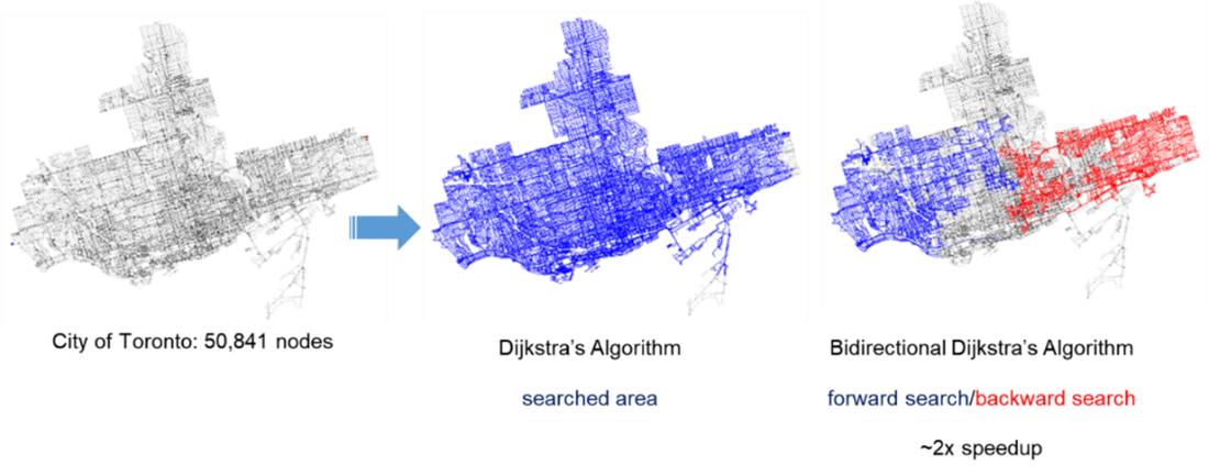
Bidirectional Dijkstra

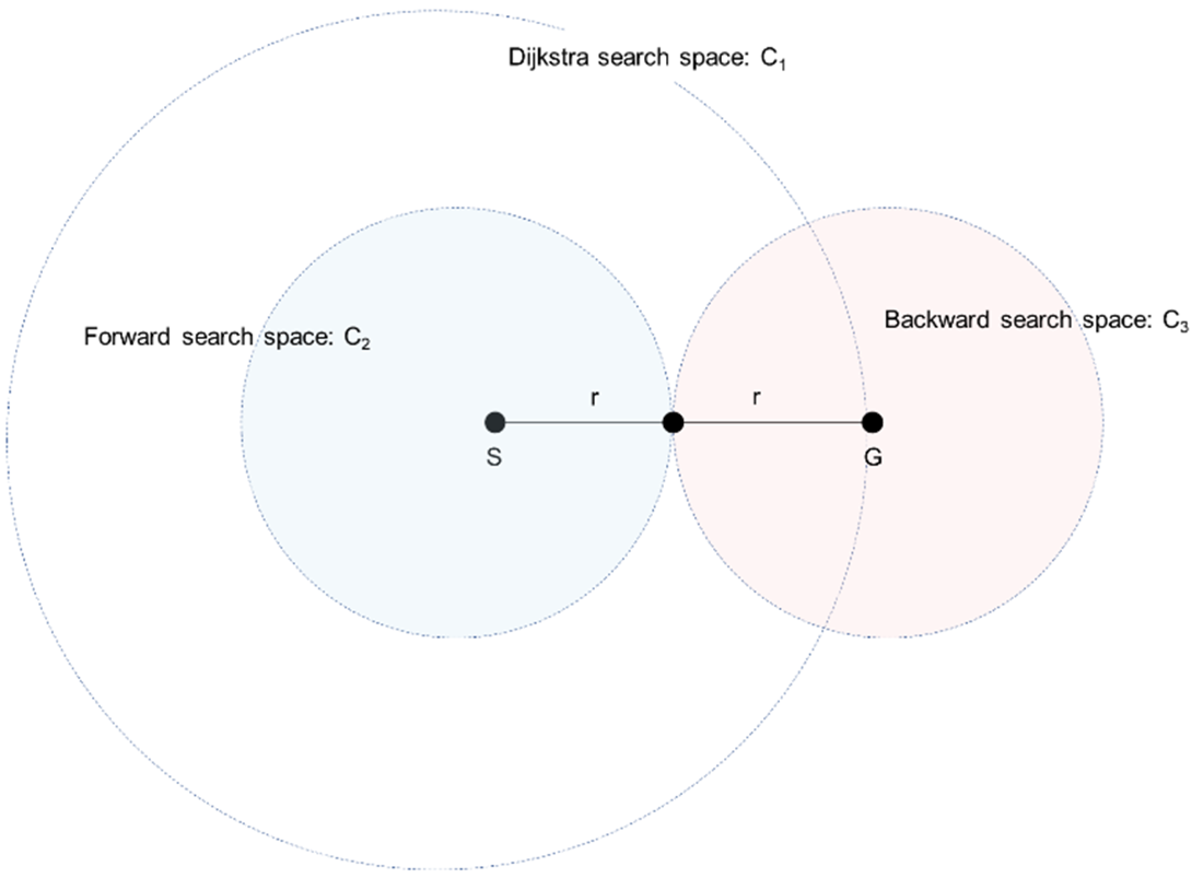
Dijkstra vs Bidirectional Dijkstra. Blue represents the forward exploration, while red shows the backward exploration.

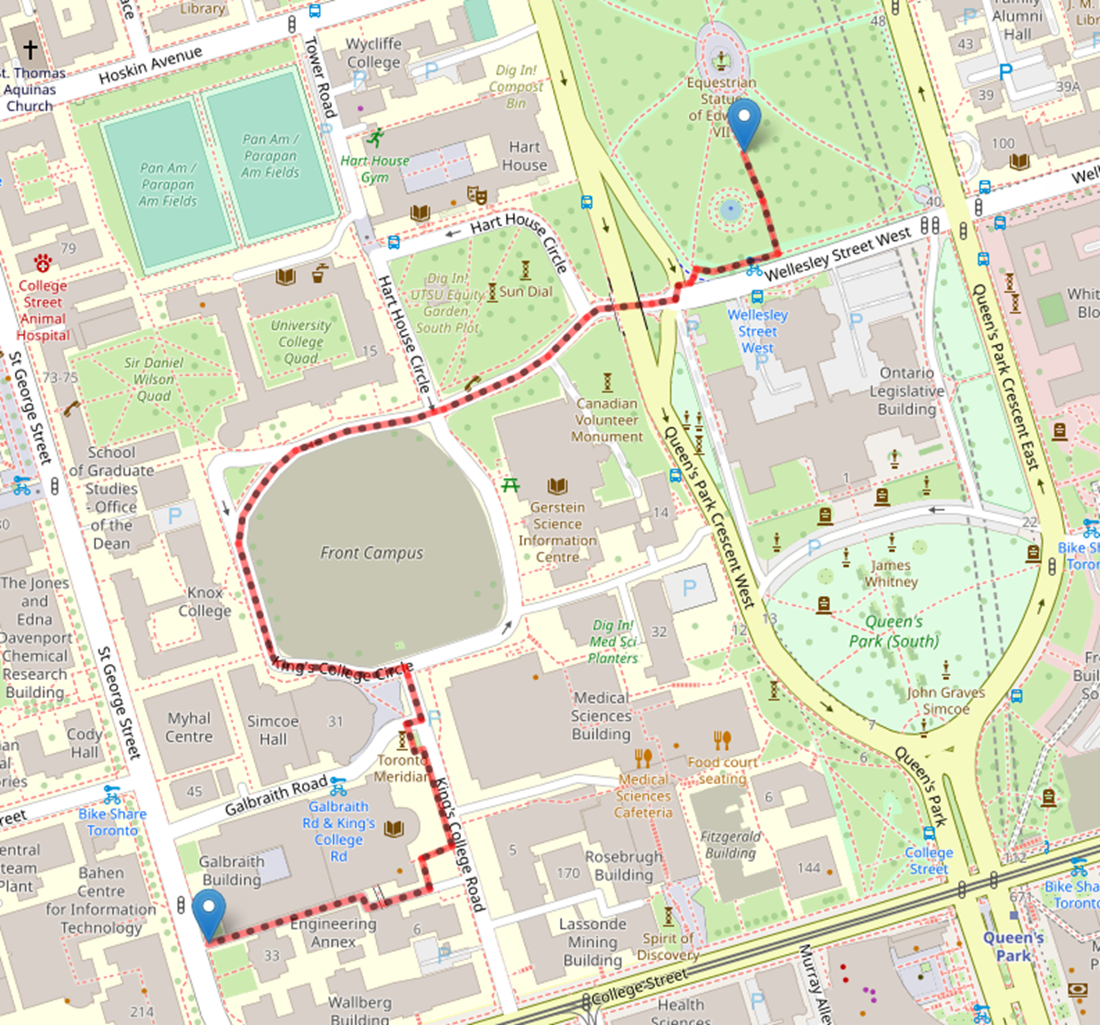
BFS routing using Python. BFS searches each layer first, before moving to the next. This works best for graphs that are not very broad and has a solution located near the root node.

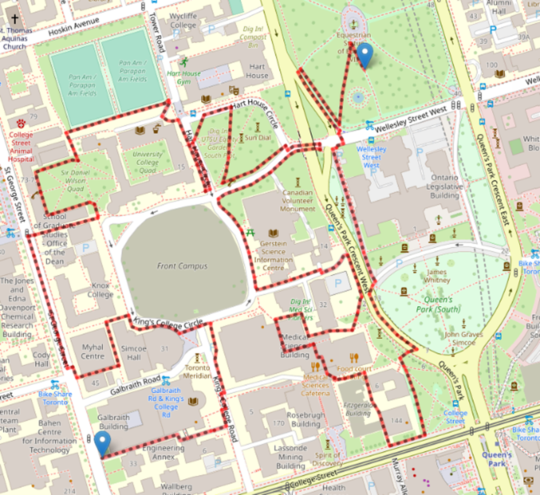
DFS routing using Python. DFS searches as deep as possible in the graph before “backtracking”. This works best when the graph is not very deep, and solutions are located further away from the root node.

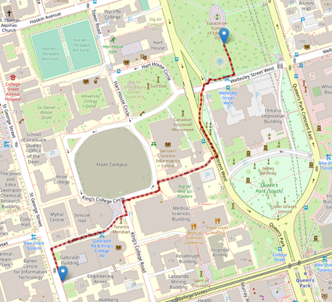
Dijkstra’s, UCS, and Bidirectional Dijkstra’s routing. All three of these algorithms will produce the same solution (optimal routing), but handle memory usage and node exploration differently.

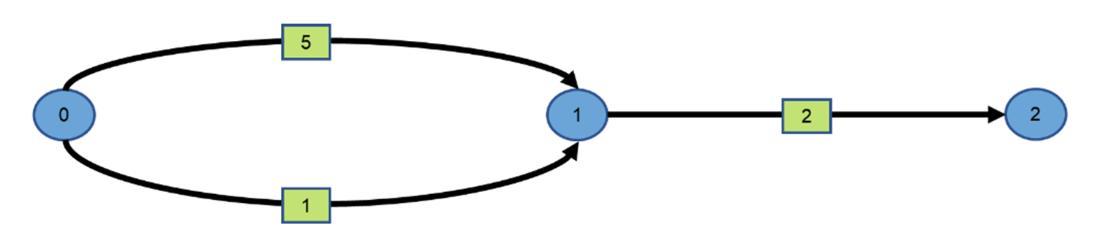
Parallel edges may be problematic as finding the shortest path depends on which parallel edge was selected during graph exploration.

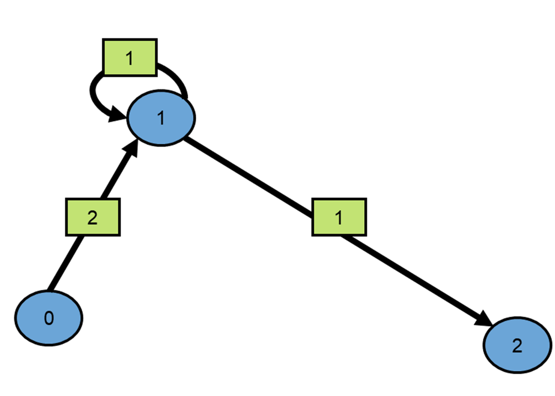
Self-loops may disrupt the chain of “parent-child nodes”, which prevents retracing the route after a solution has been found.

• Conventional graph search algorithms (blind and informed search algorithms) are deterministic search algorithms that explore a graph either for general discovery or for explicit search.
• Graph is a non-linear data structure consisting of vertices and edges.
• Blind/uninformed search is a search approach where no information about the search space is used.
• Breadth-first Search (BFS) is a graph traversal algorithm that examines all the nodes in a search tree on one level before considering any of the nodes on the next level.
• Depth-first Search (DFS) is a graph traversal algorithm that first explores nodes going through one adjacent of the root, then next adjacent until it finds a solution or until it reaches a dead-end.
• Depth-limited Search (DLS) is a constrained DFS with a predetermined depth limit to prevent exploring paths that are too long in a search tree with infinite depth.
• Iterative Deepening Search (IDS) or Iterative Deepening Depth First Search (IDDFS) combines DFS's space efficiency and BFS's fast search by incrementing the depth limit until the goal is reached.
• Dijkstra's algorithm solves the single-source shortest path problem for a weighted graph with non-negative edge costs.
• Uniform-cost Search (UCS) is a variant of Dijkstra's algorithm that uses the lowest cumulative cost to find a path from the source to the destination. It is equivalent to the BFS algorithm if the path cost of all edges is the same.
• Bidirectional Search (BS) is a combination of forward and backward search. It searches forward from the start and backward from the goal simultaneously.
• Selecting a search algorithm involves determining the target balance between time complexity, space complexity, and prior knowledge about the search space, among other factors.
• As you progress to Chapter 4, you will start to learn about informed search algorithms where additional information or heuristic rules are used during the search.

FAQ