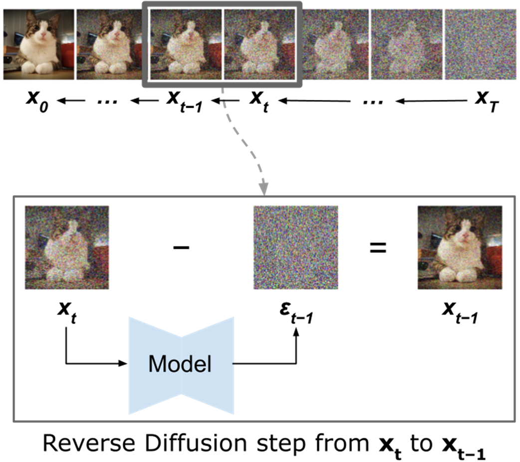
Reverse Diffusion is the generative core of diffusion models: starting from pure noise, the model iteratively removes noise step by step to reveal coherent images that reflect the training data distribution. The chapter contrasts this with Forward Diffusion, explains the intuition (progressively uncovering structure), and details how the model learns to predict the noise present at each timestep so it can be subtracted reliably. A carefully chosen noise schedule guides the process, and a small stochastic term is retained during sampling to promote diversity and avoid mode collapse. Training teaches the network to estimate the added noise at random timesteps using a simple mean squared error objective; inference chains these predictions from high to low timesteps to synthesize images.
The chapter centers noise prediction on a U-Net backbone whose encoder-decoder design with skip connections captures both global context and fine detail—crucial for accurate denoising. Time step conditioning is introduced via sinusoidal embeddings injected into the network so the model adapts its strategy across noise levels, focusing on broad structure early and fine details later. This conditioning improves accuracy and efficiency, enables flexibility in sampling (such as step skipping), and ties together the denoising and stochastic components governed by the beta/alpha schedules and their cumulative products.
To make the ideas concrete, the chapter implements a DDPM in PyTorch on MNIST: defining the beta schedule and closed-form terms, constructing a time-conditioned U-Net, applying forward and reverse diffusion, training with uniform timestep sampling and MSE on noise, and sampling by iteratively denoising from Gaussian noise, followed by qualitative evaluation (with mentions of common quantitative metrics). It closes by comparing DDPMs with VAEs and GANs: VAEs train stably but can blur; GANs generate sharp outputs quickly but may suffer instability and mode collapse; DDPMs offer stable training and high-quality, diverse samples at the cost of slower iterative generation—an increasingly favorable trade-off that powers modern text-to-image systems.
Reverse Diffusion
U-Net network
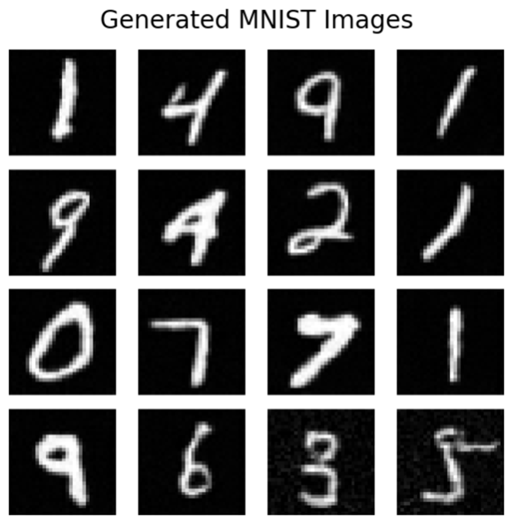
MNIST images generated by our DDPM
Summary
Forward Diffusion Process:
Gradually adds noise to data samples over a series of steps
Transforms structured data into unstructured noise
Defined by a carefully chosen noise schedule
Reverse Diffusion Process:
Learns to gradually remove noise from a noisy data
Generates new data by iteratively denoising random noise
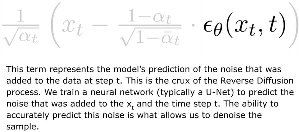
Requires a learned model to predict and remove noise at each step
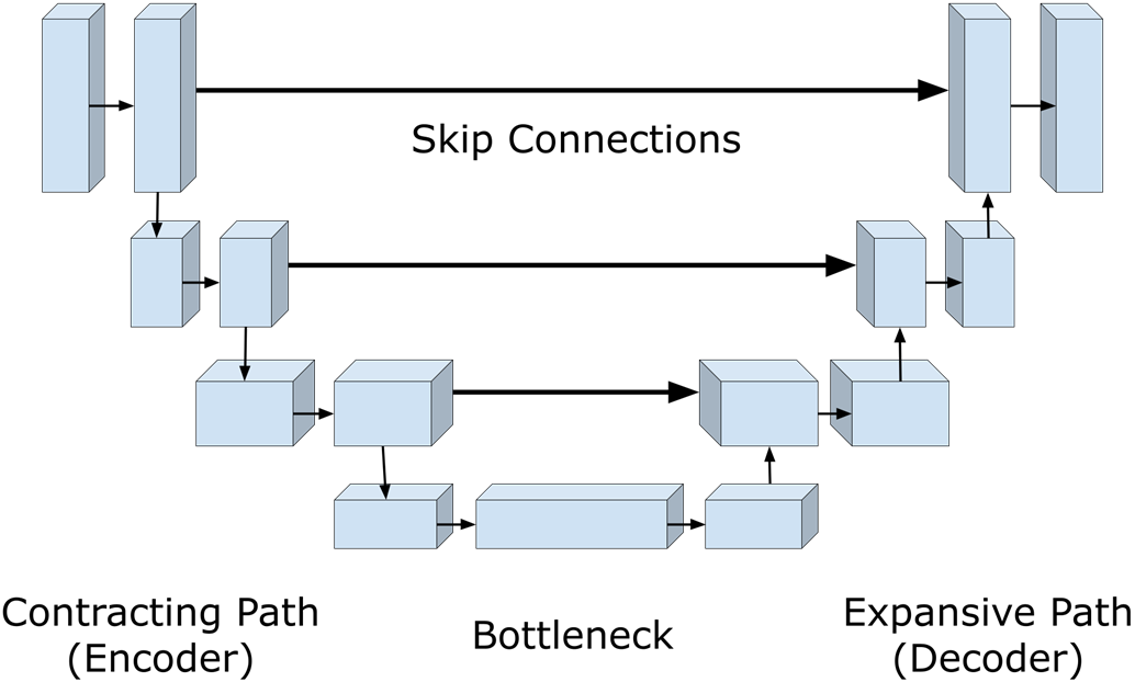
U-Net Architecture:
Crucial for effective noise prediction in DDPMs
Features a symmetric encoder-decoder structure with skip connections
Allows the network to capture both fine-grained details and broader context
Time Step Conditioning:
Enables the model to adapt its denoising behavior based on the current diffusion step
Implemented through sinusoidal position encodings
Crucial for the model’s ability to handle different noise levels
DDPM Training:
Involves forward diffusion to create noisy samples and reverse diffusion to denoise
Uses a simple mean squared error loss between predicted and actual noise
Generally more stable than adversarial training (as in GANs)
DDPM Sampling (Generation):
Starts from pure noise and iteratively applies the reverse diffusion process
More computationally intensive than sampling from VAEs or GANs
Produces high-quality and diverse samples
Comparison with VAEs and GANs:
DDPMs often produce higher quality and more diverse samples than VAEs
DDPMs can match or exceed GAN quality while offering more stable training
DDPMs are slower in generating samples compared to both VAEs and GANs
FAQ
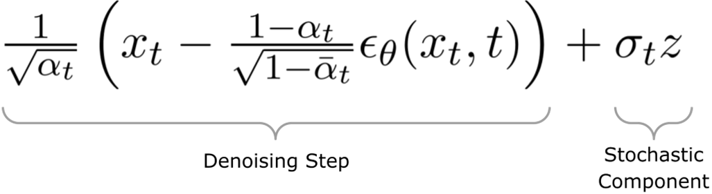
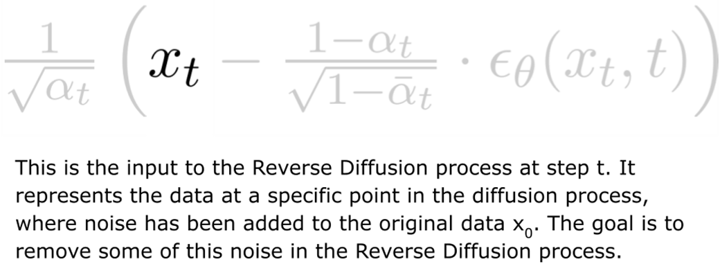
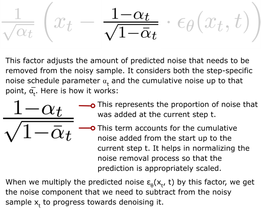
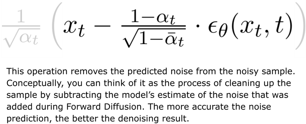
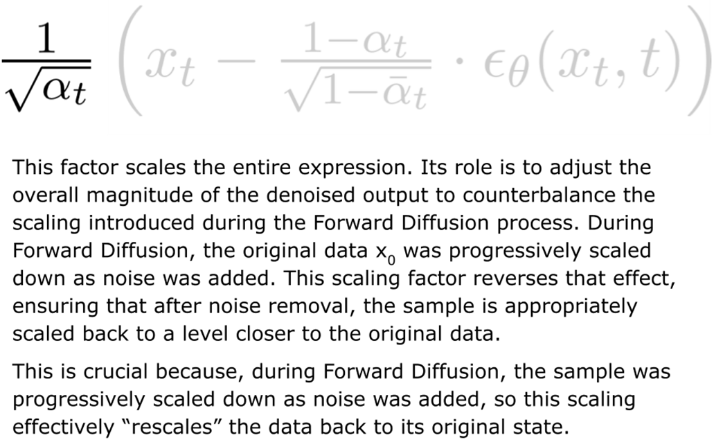
What is Reverse Diffusion, and how does it relate to Forward Diffusion?Reverse Diffusion inverts Forward Diffusion. While Forward Diffusion adds Gaussian noise to a clean sample x0 over T steps to produce xT (pure noise), Reverse Diffusion iteratively removes that noise: starting from xT and using a learned model to predict and subtract the noise at each timestep to recover x0. This is how diffusion models generate new images from random noise.How does the Reverse Diffusion update (Equation 5.2) work?Equation 5.2 updates xt to xt−1 with two parts:
- Denoising term: uses the model’s noise prediction εθ(xt, t) and step-dependent scalings (αt, α̅t) to subtract the estimated noise proportionally to how much was added in the forward process.
- Stochastic term: adds σtz (with z ~ N(0, I)) to maintain diversity and correct statistical properties.
Together, these refine structure while preserving probabilistic sampling.Why does the Reverse Diffusion step add noise (the stochastic component)?The controlled noise σtz is crucial to:
- Avoid mode collapse by allowing multiple denoising paths.
- Improve generalization by preventing overfitting to a single deterministic path.
- Increase realism and diversity by preserving the probabilistic nature of the process.
σt typically decreases as t→0 so late steps are less noisy.What exactly does the model learn during training, and what loss is used?During training, the model learns to predict the noise ε added at any timestep t. We:
- Sample x0, pick t ~ Uniform(1, T), generate xt via the closed-form forward noising equation.
- Train the network to predict ε from (xt, t).
- Use mean squared error loss L = E[||ε − ε̂θ(xt, t)||²]. Accurate noise prediction enables effective reverse denoising.How does inference (sampling) generate new images from noise?Sampling proceeds by:
- Initializing xT ~ N(0, I).
- For t = T, T−1, …, 1: predict εθ(xt, t) and apply Equation 5.2 to obtain xt−1.
- Output x0 as the generated image.
This iterative process transforms noise into a coherent sample from the learned data distribution.Why is a U-Net used for noise prediction in diffusion models?U-Net is effective because:
- Encoder–decoder with skip connections captures multi-scale context (global structure) and preserves fine details.
- Skip connections restore spatial precision lost during downsampling.
- Its symmetric “U” design naturally supports image-to-image mapping tasks like denoising.
These properties make it well-suited to predict ε at varying noise levels.What is timestep conditioning/embedding, and how is it implemented?Timestep conditioning informs the network “how noisy” the input is. Implementation:
- Encode t into a high-dimensional vector using sinusoidal embeddings.
- Inject the embedding into the U-Net (e.g., added as channels or injected at multiple layers).
Benefits:
- Specializes denoising behavior per noise level.
- Improves learning efficiency and quality.
- Enables flexibility (e.g., step skipping or adaptive schedules during inference).How does the noise schedule βt influence training and sampling?The schedule βt (and derived αt, α̅t) controls how quickly noise is added in forward diffusion and thus how denoising scales are set in reverse:
- Typically increases over time to ensure gradual corruption.
- Affects stability, sample quality, and the difficulty of predictions at each step.
- Precomputing α products enables closed-form xt sampling and efficient training.How do DDPMs compare with VAEs and GANs?Trade-offs:
- Quality/diversity: DDPMs produce sharp, diverse samples; often rival or surpass GANs on benchmarks; VAEs can be blurrier but cover modes well.
- Speed: VAEs and GANs sample in a single pass; DDPMs require many iterative steps (slower).
- Stability: DDPMs train stably with a simple MSE objective; GANs can be unstable; VAEs are generally stable.What are key practical tips for implementing a DDPM in PyTorch?Tips:
- Normalize data to [-1, 1] and clamp outputs accordingly.
- Sample timesteps t uniformly per batch item during training.
- Precompute α, α̅, and related terms for efficiency and numerical stability.
- Use GPU if available; keep shapes consistent when broadcasting timestep-dependent scalars.
- Inject timestep embeddings throughout the U-Net.
- Expect slower sampling; consider fewer steps or acceleration methods if needed.