4 Diffusion Models: Forward Diffusion
Diffusion models are a class of generative models that create images by moving between order and randomness through many small steps. Unlike VAEs and GANs that map directly from latent codes to images, diffusion models rely on a two-phase mechanism: a Forward Diffusion phase that gradually corrupts data with noise, and a Reverse Diffusion phase that learns to remove it. This chapter builds intuition for that process—drawing on ideas like Brownian motion and probabilistic views of images—emphasizing that coherent, high-quality images occupy a tiny manifold within an astronomically large space of possible pixel grids. By understanding how structure is lost in a controlled way, we set up the learning task of reconstructing it.
The Forward Diffusion process incrementally adds Gaussian noise over T steps, transforming an original sample x0 into xT that is nearly isotropic Gaussian noise. It is a Markov process with a predefined variance schedule βt that controls how much noise is added at each step; schedules are typically small at the start and larger later (e.g., linear or cosine), enabling the model to learn fine details at low noise and broader structure at high noise. This intentional corruption simplifies the intractable data distribution into a tractable one while remaining reversible in principle. Mathematically, the process is designed so the distribution approaches Gaussian as t increases, and a closed-form expression allows direct sampling of any intermediate xt from x0 without iterating through all prior steps, improving efficiency. Visualized in 1D, Forward Diffusion smooths complex, multimodal densities into a single-peaked Gaussian, illustrating how structure is progressively washed out.
Practically, Forward Diffusion supplies the training signals for learning the reverse mapping: the model is trained to predict and remove the noise added at each step, enabling it to trace a path from high-entropy noise back to low-entropy, coherent images. This design distills coherence from chaos and underpins the strong sample quality, diversity, and training stability observed with DDPMs. With the foundations, terminology, and motivation established here—why Gaussian noise, how βt shapes learning, and how closed-form skipping aids computation—the stage is set for the next chapter’s detailed treatment of Reverse Diffusion and a hands-on construction of denoising diffusion models from scratch.
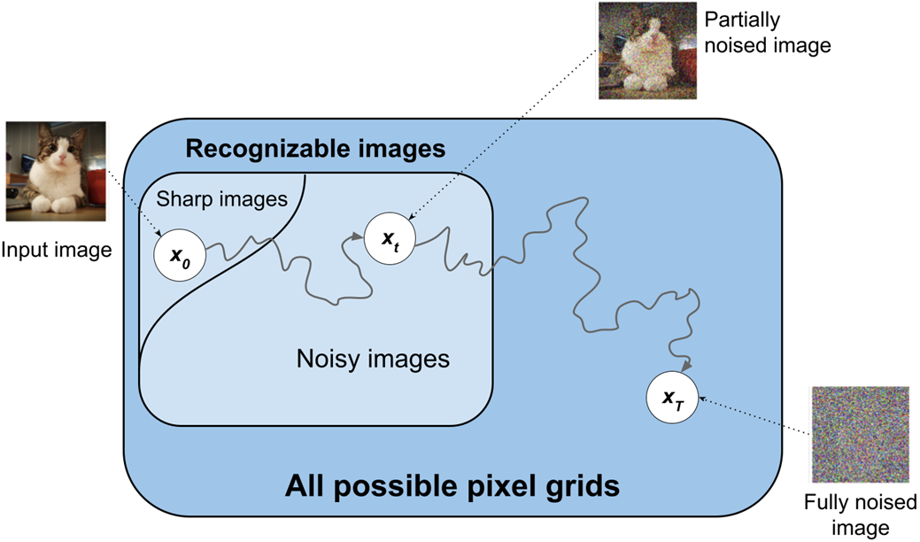
[1] Example of Forward and Reverse diffusion.
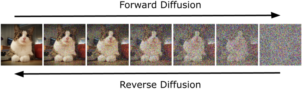
Illustration of the Forward Diffusion process.
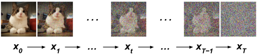
Illustration of the noise addition step in a single step t in during the Forward Diffusion phase, transforming image xt into xt+1 by adding the noise εt.
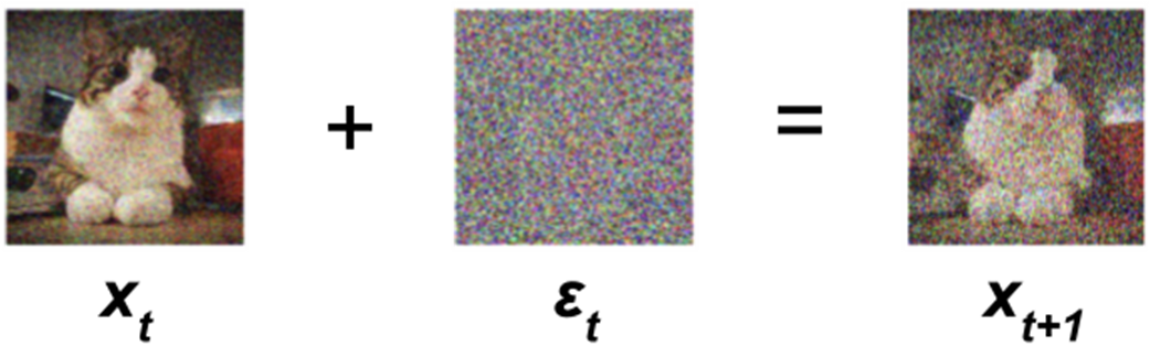
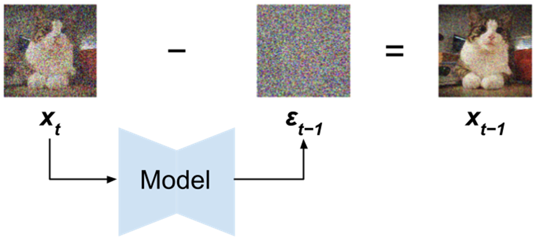
Illustration of noise removal via Reverse Diffusion. Given a noisy image xt, the Reverse Diffusion model learns to predict εt-1. By subtracting this noise, the model aims to recover the previous image state, xt-1.
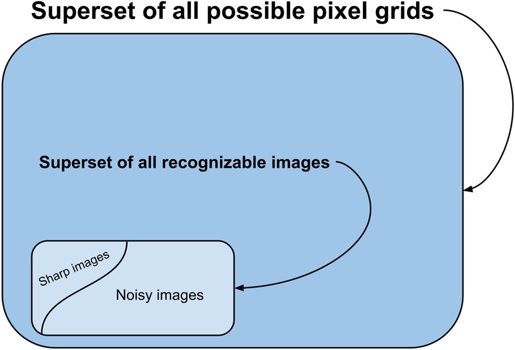
Conceptual visualization of the universe of all possible images.
Conceptual illustration of Diffusion in the pixel space. Diffusion Models learn the complex distribution of real images by first adding noise to these images and then learning to reverse this process. Through training, they effectively map the journey from disorder (random noise) to order (structured, recognizable imagery).
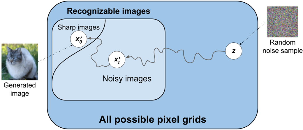
Using Diffusion to synthesize new images.
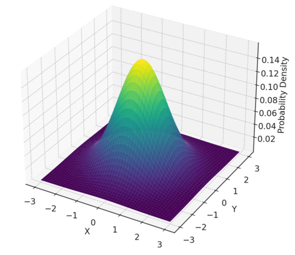
Isotropic Gaussian distribution over 2-dimensions. Characteristic of an Isotropic Gaussian, the distribution exhibits uniform variance in every direction, manifesting in a perfectly symmetrical shape around its mean. This uniformity implies that the data points spread out from the center with equal probability in all planar directions, exhibiting isotropy.
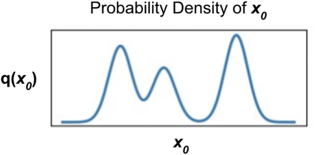
[2] Probability density function of 1D data. This figure shows a Probability Density Function (PDF) for 1D data, with the x-axis representing the data coordinates and the y-axis indicating probability density. A complex, multimodal (having multiple peaks) distribution exemplifies how certain x-coordinates are more likely to host data points, based on the peak heights. That is, the higher the PDF curve denoted as q(x0), the more likely it is that a randomly sampled datapoint would have an x-coordinate near the peak.
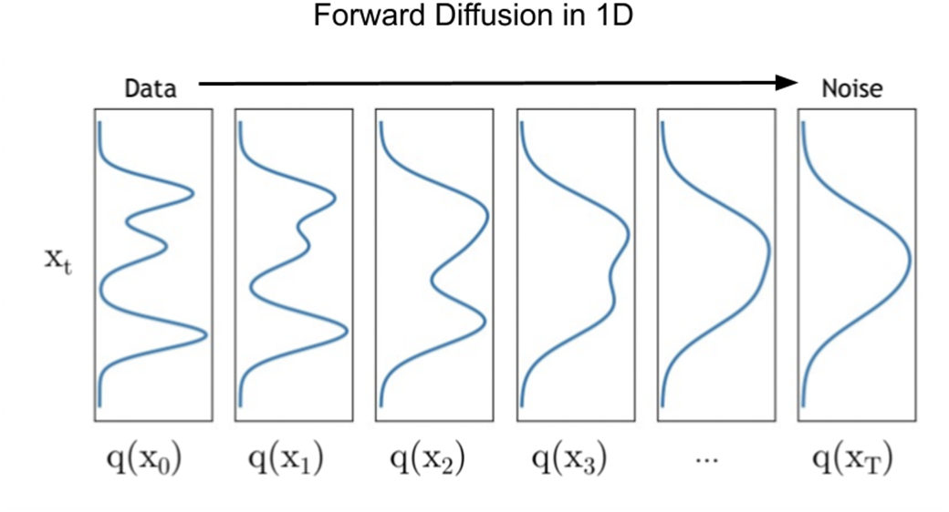
[3] Evolution of 1D data distribution via Forward Diffusion. This figure illustrates the transformation of the input data’s probability density, q(x0), into a Standard Normal Distribution, q(xT) via Forward Diffusion. It illustrates the progressive smoothing of the original data distribution’s characteristics through gradual Gaussian noise addition until they align with those of a Gaussian distribution.
Summary
- Diffusion models: A class of generative models that gradually transform simple distributions (e.g., Gaussian noise) into complex data distributions (e.g., images) through a process of iterative denoising, effectively learning to reverse the diffusion process. Diffusion models operate through a two-phase process: Forward Diffusion to introduce noise, and Reverse Diffusion to remove noise and reconstruct images.
- Forward Diffusion: The Forward Diffusion process systematically adds noise to the original data over a series of steps, moving it towards a distribution that is easier to model and sample from, typically Gaussian noise. This process is designed to be reversible, setting the stage for the Reverse Diffusion process where the model learns to denoise or reconstruct the original data from noise.
- Gaussian noise: Gaussian noise, or normally distributed noise, is the type of noise typically added during the Forward Diffusion process, characterized by its bell-shaped probability distribution. Gaussian noise is favored because of its well-understood properties and mathematical tractability, making it ideal for the controlled degradation of data.
- Variance schedule: The variance schedule is a predefined sequence of values that dictate the amount of noise added at each step of the Forward Diffusion process. It ensures that the noise addition is both gradual and controlled, preventing the data from becoming too corrupted too quickly. This plays a key role in the reversibility of the diffusion process, allowing the model to accurately learn how to reverse the noise addition during the Reverse Diffusion phase.
FAQ
What is the Forward Diffusion process in diffusion models?
The Forward Diffusion process gradually adds noise to an original image x0 over T timesteps, producing increasingly noisy versions xt until the data becomes indistinguishable from random (Gaussian) noise at xT. This controlled corruption defines a path the model later learns to reverse.Why do we add noise during Forward Diffusion?
Adding noise reduces the complexity of the original data distribution, transforming it into a simple, tractable Gaussian distribution. This simplification makes sampling easier and sets up a reversible process the model can learn to invert during generation.How do the Forward and Reverse Diffusion phases differ?
- Forward Diffusion: incrementally corrupts data by adding noise, moving from structure to noise (x0 → xT).- Reverse Diffusion: learns to remove noise step by step, moving from noise to structure (xT → x0) to reconstruct or synthesize coherent images.
What does it mean that the Forward Diffusion process is Markovian?
It means each noisy state xt depends only on the immediate previous state xt−1 (and the current noise), not on earlier steps. This property simplifies analysis and is key to designing a reversible denoising process.Why is Gaussian (especially isotropic Gaussian) noise chosen?
Gaussian noise is used because of its symmetry, mathematical tractability, and the Central Limit Theorem. An isotropic Gaussian has equal variance in all directions, yielding a simple, well-understood target distribution for the end of the forward process.How is noise added at each timestep?
At each step t, a small, scheduled amount of Gaussian noise ε is added to the previous sample xt−1. The addition is scaled by a variance schedule βt so that corruption is gradual—small at first and larger later—preventing the data from becoming noise too quickly.What is the variance schedule βt and why does it matter?
βt controls how much noise is added at each step. It typically starts near zero and increases over time. Its shape significantly affects training dynamics and sample quality. Common choices:- Linear schedule: variance increases at a constant rate.
- Cosine schedule: variance increases nonlinearly, with smoother changes at the beginning and end.