2 Variational Autoencoders (VAEs)
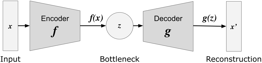
This chapter introduces autoencoders as self-supervised neural networks that learn compact, meaningful representations by reconstructing their inputs. It explains the encoder–decoder architecture, the notion of a latent space, and why compressing through a bottleneck yields salient features useful for tasks such as dimensionality reduction, denoising, anomaly detection, and feature learning. While traditional autoencoders excel at reconstruction, the chapter motivates the need for truly generative models that can sample new data, setting the stage for Variational Autoencoders (VAEs).
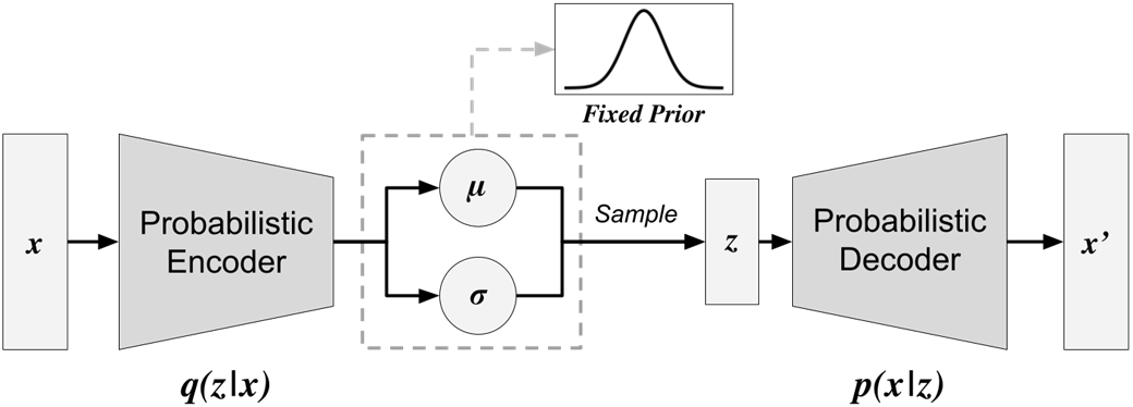
VAEs extend autoencoders by making the latent space probabilistic: the encoder predicts parameters of a distribution (typically mean and variance of a Gaussian) for each input, and the decoder reconstructs data from latent samples. Training balances two objectives—a reconstruction loss for fidelity and a regularization term that aligns latent distributions with a simple prior—enabled by the reparameterization trick so gradients can flow through sampling. The chapter walks through a practical PyTorch implementation on MNIST, demonstrates evaluation via reconstructions and random sampling, and shows how latent space interpolation produces smooth, semantically coherent transitions that reflect a continuous, well-structured representation.
Building on this foundation, the chapter presents β-VAE, which introduces a hyperparameter to weight the regularization term and promote disentangled latent factors. Increasing β typically trades some reconstruction accuracy for more interpretable, factorized representations where individual latent dimensions control distinct attributes, enabling controlled generation and analysis. The discussion underscores the broader implications: from reliable compression and generation to human-interpretable representations, charting a progression from basic autoencoders to VAEs and β-VAEs as powerful tools for image generation and representation learning.
Autoencoder model architecture
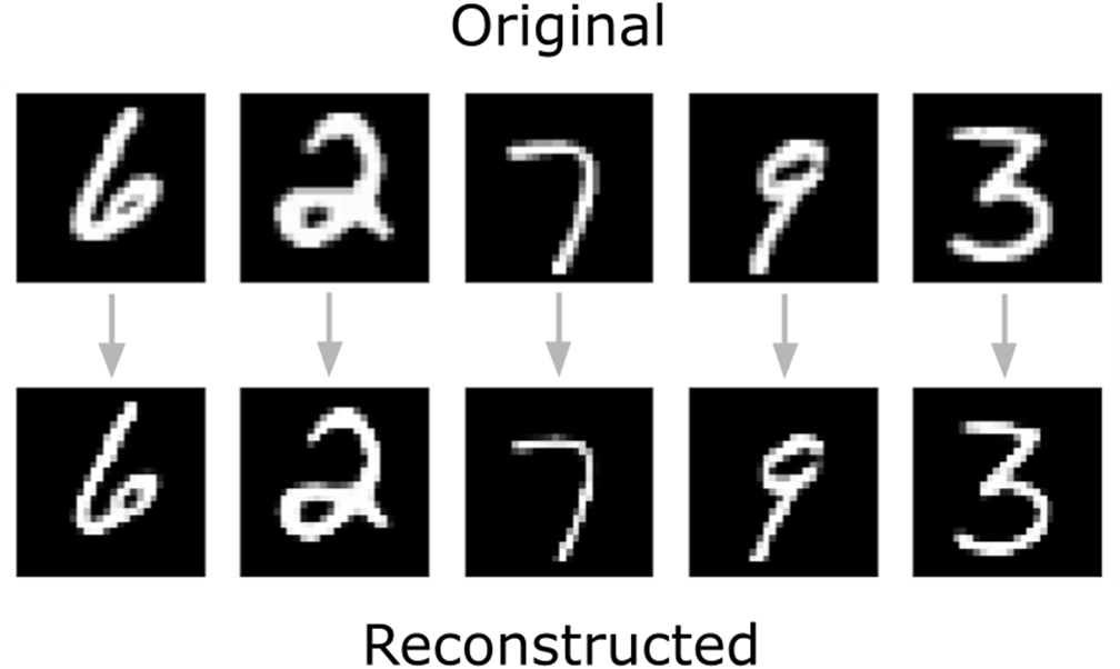
Comparison of original MNIST digits (top row) with their autoencoder reconstructions (bottom row)
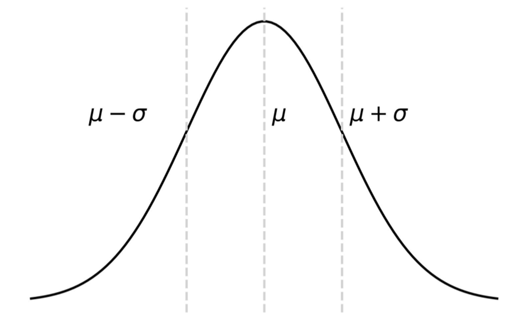
Normal (Gaussian) distribution. This figure illustrates a bell-shaped curve representing a Normal distribution denoted by N(μ, σ): μ represents the mean or average of the distribution. σ represents the standard deviation, a measure of how spread out the values are around the mean in the distribution.
VAE model architecture
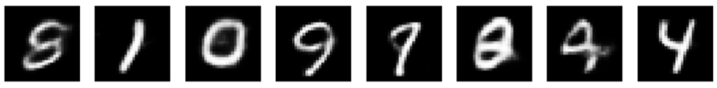
Randomly generated MNIST digits created by VAE
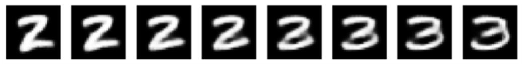
Latent space interpolation involves selecting two distinct points in the latent space, which represent different latent encodings, and creating a series of intermediate points between them. By feeding interpolated latent vectors into the VAE’s decoder, we can reconstruct the data corresponding to each point. This allows us to observe how the data transitions as we move from one latent representation to another.
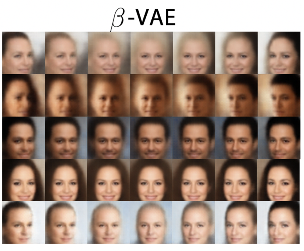
[5] Disentangled latent variables in β-VAEs
Summary
- Autoencoders: Neural network architectures used to learn efficient codings of the input data; autoencoders have an encoder-decoder structure where the encoder compresses the input and the decoder reconstructs it, aiming to match the original.
- Latent space: The hidden, compact representation of data, where autoencoders compress the input data. It represents the essential features learned from the data, which are crucial for the reconstruction or generation of new data instances.
- Variational autoencoders (VAEs): An advanced type of autoencoder that learns the distribution of the data in the latent space. Unlike traditional autoencoders, VAEs are generative models that can generate new instances that resemble the input data by sampling from the learned distribution in the latent space.
- Reparameterization trick: The reparametrization trick is a method used in VAEs to enable backpropagation through random processes by decoupling the sampling operation from the model’s parameters.
- Beta-VAEs (β-VAEs): An extension of the standard VAE, introducing a hyperparameter β (beta) to control the trade-off between accurate reconstruction and adherence to the latent space’s probabilistic distribution, often leading to improved disentanglement of features in the latent space.