4 Optimizing the training process: Underfitting, overfitting, testing, and regularization
This chapter focuses on how to steer training toward models that generalize well, framing two common pitfalls—underfitting and overfitting—as problems of mismatched complexity. Underfitting arises when a model is too simple to capture the signal; overfitting occurs when a model is so flexible it memorizes noise. Using polynomial regression as a running example, the chapter shows how training error reliably drops as complexity increases, while performance on unseen data follows a U-shaped pattern: high for overly simple models, lowest at a “just right” complexity, and high again for models that overfit. The practical takeaway is that model selection must be driven by generalization, not by training error alone.
To measure generalization, the chapter emphasizes disciplined data splitting and the “golden rule”: never use test data to make modeling decisions. It introduces a three-way split—training (to fit parameters), validation (to tune hyperparameters and select models), and testing (to assess final quality)—and discusses typical proportions. The model complexity graph, which plots training and validation error against a complexity knob (such as polynomial degree), helps visualize where a model stops underfitting and starts overfitting. While the lowest validation error is the primary criterion, the chapter encourages favoring a simpler model when its validation performance is nearly as good, reflecting a preference for parsimony and robustness.
Regularization provides a complementary route to control complexity during training by augmenting the objective with a penalty on model size. Complexity is quantified via the L1 or L2 norms of the coefficients, yielding lasso (L1) and ridge (L2) regression, respectively, with a regularization strength λ that trades off fit and simplicity (chosen via validation). L1 tends to drive many coefficients exactly to zero, aiding feature selection and interpretability; L2 shrinks all coefficients without making most of them vanish, promoting smoother, more stable solutions. In practice, unregularized models can fit training data perfectly yet fail on new data, whereas appropriately regularized models capture the essential structure (for example, a clean quadratic trend) and deliver strong test performance. The chapter closes with guidance: select complexity with validation, prefer the simplest near-optimal model, use L1 when you want sparsity across many features, and use L2 when you expect most features to matter but need them kept small.

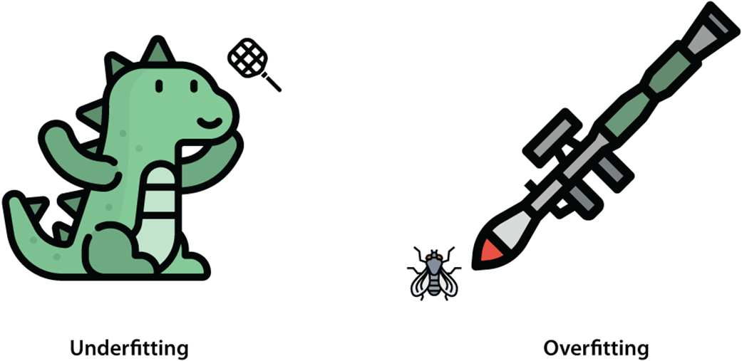
Underfitting and overfitting are two problems that can occur when training our machine learning model. Left: Underfitting happens when we oversimplify the problem at hand, and we try to solve it using a simple solution, such as trying to kill Godzilla using a fly swatter. Right: Overfitting happens when we overcomplicate the solution to a problem and try to solve it with an exceedingly complicated solution, such as trying to kill a fly using a bazooka.
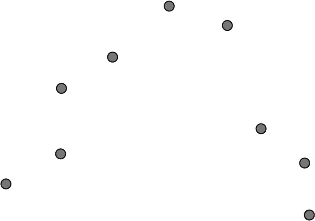
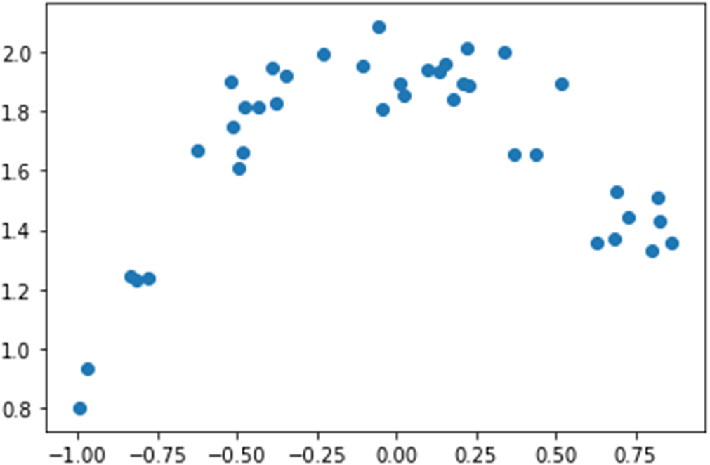
In this dataset, we train some models and exhibit training problems such as underfitting and overfitting. If you were to fit a polynomial regression model to this dataset, what type of polynomial would you use: a line, a parabola, or something else?
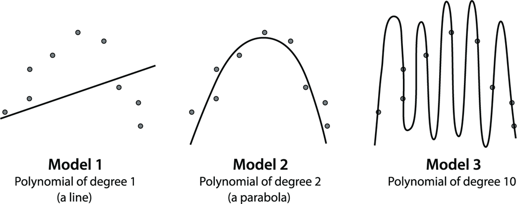
Fitting three models to the same dataset. Model 1 is a polynomial of degree 1, which is a line. Model 2 is a polynomial of degree 2, or a quadratic. Model 3 is a polynomial of degree 10. Which one looks like the best fit?
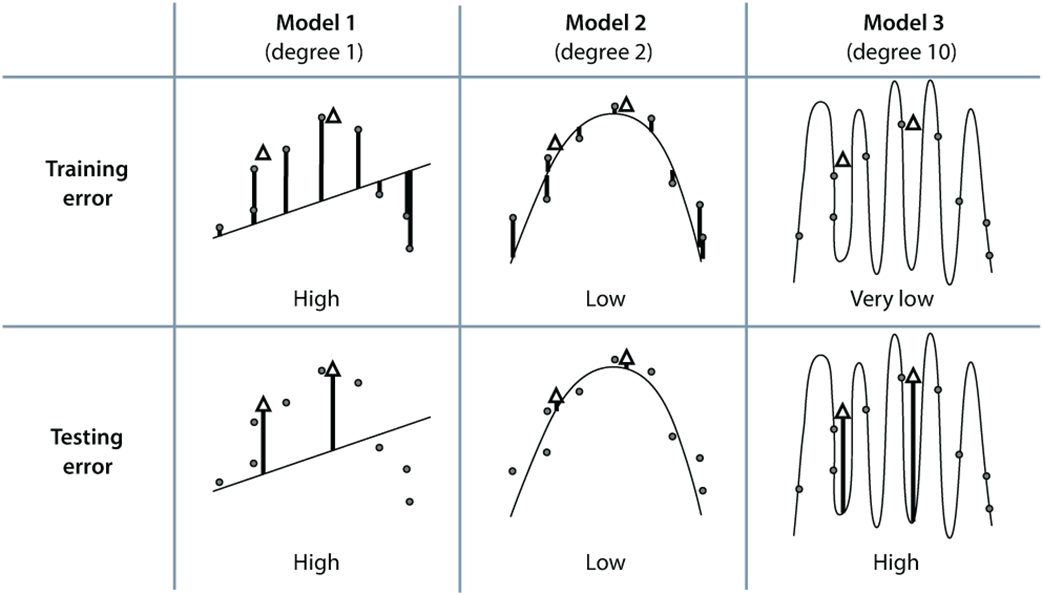
We can use this table to decide how complex we want our model. The columns represent the three models of degree 1, 2, and 10. The rows represent the training and the testing error. The solid circles are the training set, and the white triangles are the testing set. The errors at each point can be seen as the vertical lines from the point to the curve. The error of each model is the mean absolute error given by the average of these vertical lengths. Notice that the training error goes down as the complexity of the model increases. However, the testing error goes down and then back up as the complexity increases. From this table, we conclude that out of these three models, the best one is model 2, because it gives us a low testing error.
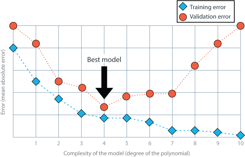
The model complexity graph is an effective tool to help us determine the ideal complexity of a model to avoid underfitting and overfitting. In this model complexity graph, the horizontal axis represents the degree of several polynomial regression models, from 0 to 10 (i.e., the complexity of the model). The vertical axis represents the error, which in this case is given by the mean absolute error. Notice that the training error starts large and decreases as we move to the right. This is because the more complex our model is, the better it can fit the training data. The validation error, however, starts large, then decreases, and then increases again—very simple models can’t fit our data well (they underfit), whereas very complex models fit our training data but not our validation data because they overfit. A happy point in the middle is where our model neither underfits or overfits, and we can find it using the model complexity graph.
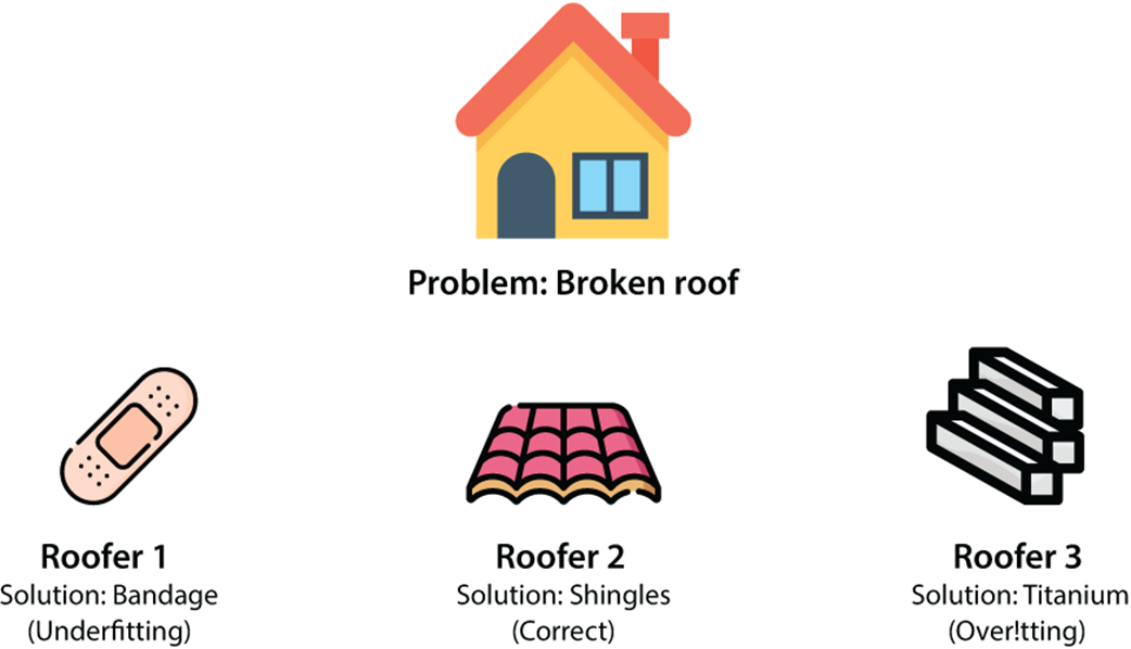
An analogy for underfitting and overfitting. Our problem consists of a broken roof. We have three roofers who can fix it. Roofer 1 comes with a bandage, roofer 2 comes with roofing shingles, and roofer 3 comes with a block of titanium. Roofer 1 oversimplified the problem, so they represent underfitting. Roofer 2 used a good solution. Roofer 3 overcomplicated the solution, so they represent overfitting.
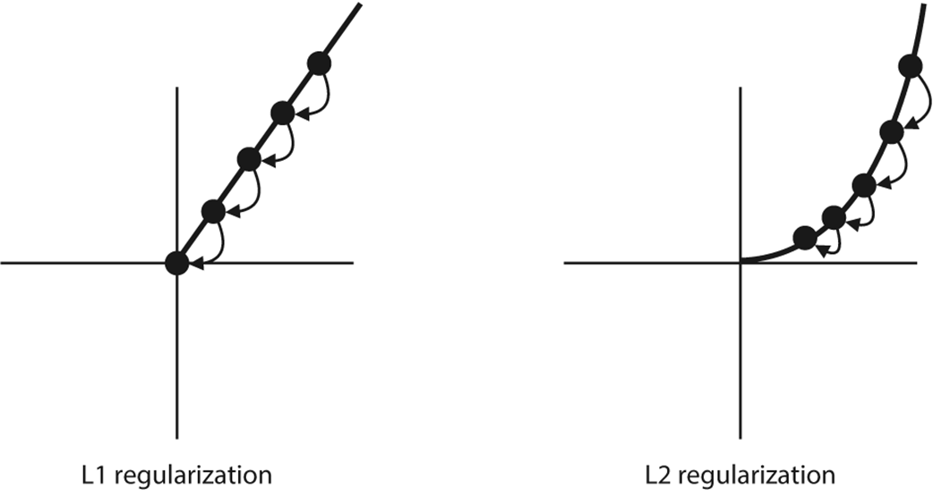
Both L1 and L2 shrink the size of the coefficient. L1 regularization (left) does it much faster, because it subtracts a fixed amount, so it is likely to eventually become zero. L2 regularization takes much longer, because it multiplies the coefficient by a small factor, so it never reaches zero.
The dataset. Notice that its shape is a parabola that opens downward, so using linear regression won’t work well. We’ll use polynomial regression to fit this dataset, and we’ll use regularization to tune our model.
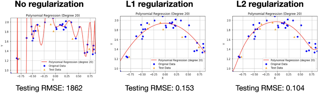
Three polynomial regression models for our dataset. The model on the left has no regularization, the model in the middle has L1 regularization with a parameter of 0.01, and the model on the right has L2 regularization with a parameter of 0.01.
FAQ
What are underfitting and overfitting?
Underfitting happens when a model is too simple to capture the data patterns (high error on both training and testing). Overfitting happens when a model is too complex and memorizes the training data (low training error but high testing error). The goal is a model that fits the training data well and generalizes to unseen data.
How can I tell if my model underfits or overfits using errors?
- High training error + High testing/validation error → Underfitting
- Low training error + High testing/validation error → Overfitting
- Low training error + Low testing/validation error → Good fit
How should I split data into training, validation, and testing sets?
Use three splits to prevent leakage and tune hyperparameters safely:
- Training: fit model parameters
- Validation: choose models/hyperparameters
- Testing: final, one-time evaluation
Common ratios: 60-20-20 or 80-10-10 (train–val–test). Avoid using the test set for any decisions.
What is the golden rule for test data, and how is it often broken?
Golden rule: never use your testing data for training or model/hyperparameter selection. It’s often broken inadvertently by peeking at test performance to pick a model. Use a separate validation set for all choices and reserve the test set strictly for the final evaluation.
What is a model complexity graph, and how do I use it?
It plots error versus model complexity (e.g., polynomial degree):
- Training error typically decreases as complexity increases.
- Validation error usually decreases, then increases (U-shaped), revealing underfitting on the left and overfitting on the right.
Pick the complexity with the lowest validation error, possibly favoring a simpler model if its error is close.
What is regularization, and why does it help?
Regularization adds a complexity penalty to the error minimized during training: Error = Regression error + Regularization term. By discouraging overly large or numerous coefficients, it reduces model complexity and improves generalization, combating overfitting.
What are L1 and L2 norms, and how do they measure complexity?
- L1 norm: sum of absolute values of coefficients (excluding bias)
- L2 norm: sum of squared coefficients (excluding bias)
Both increase with more or larger coefficients, quantifying model complexity for regularization.
What’s the difference between lasso (L1) and ridge (L2) regression?
- Lasso (L1): drives some coefficients exactly to zero → sparse, feature selection effect
- Ridge (L2): shrinks all coefficients toward zero but rarely to exactly zero → uses all features with smaller weights
Choose L1 when you want a simpler, sparse model; choose L2 when you believe most features are relevant but need shrinkage.
What does the regularization parameter λ (alpha) do, and how do I choose it?
λ balances fit vs. simplicity: larger λ increases penalty (simpler model, risk of underfitting); λ = 0 removes regularization. Try a grid (e.g., 10, 1, 0.1, 0.01) and pick the value with the best validation performance.
How do I apply polynomial regression with regularization in scikit-learn?
Steps:
- Expand features with PolynomialFeatures(degree=d, include_bias=False).
- Split into train/validation/test.
- Fit with Lasso(alpha=...) or Ridge(alpha=...).
- Evaluate on validation; reserve test for final check.
Regularization stabilizes high-degree fits, reducing oscillations and improving test performance.
 Grokking Machine Learning, Second Edition ebook for free