5 Advanced evolutionary approaches
This chapter deepens the genetic algorithm lifecycle introduced earlier by showing how each stage—selection, encoding, crossover, mutation, and survivor choice—can be swapped or tuned to match the problem at hand. It motivates the need for alternatives when simple binary encodings or basic operators fall short, and it uses variations on the Knapsack Problem to illustrate when different representations are more natural and effective. A recurring theme is that good performance hinges not only on operator choice but also on a fitness function that faithfully captures the true objective, especially when constraints (like steady output rates) complicate evaluation.
To balance exploration and exploitation during selection, the chapter introduces strategies beyond roulette-wheel: rank selection reduces dominance by scaling probability to rank rather than raw fitness; tournament selection offers fast, tunable pressure by pitting random groups and picking local winners; and elitism preserves top performers across generations to prevent regression. Used together, these techniques help maintain diversity while steadily improving solutions, with the caveat that too much elitism can cause premature convergence to local optima.
When problem structure demands it, alternative encodings unlock better search dynamics. Real-value encoding represents continuous or multi-quantity decisions and pairs naturally with arithmetic crossover plus boundary and incremental arithmetic mutations. Order (permutation) encoding models sequences and routes, relying on permutation-preserving crossovers (such as PMX, OX, CX) and simple swap mutations. Tree encoding captures hierarchical or programmatic structures, enabling subtree crossover and node-value mutations; this underpins genetic programming, while evolutionary programming tunes parameters of fixed programs. The chapter closes by emphasizing the modularity of these choices and highlighting broader applications—from neural network weight tuning to circuit and molecular design—where evolutionary algorithms excel.
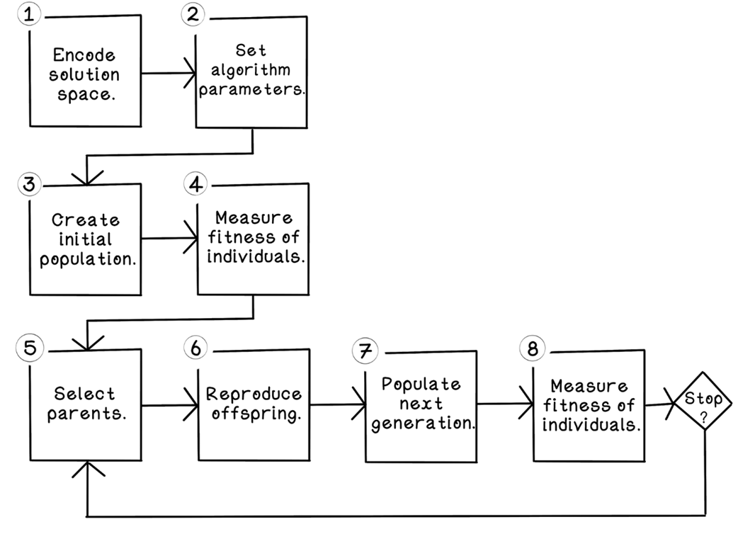
Genetic algorithm life cycle
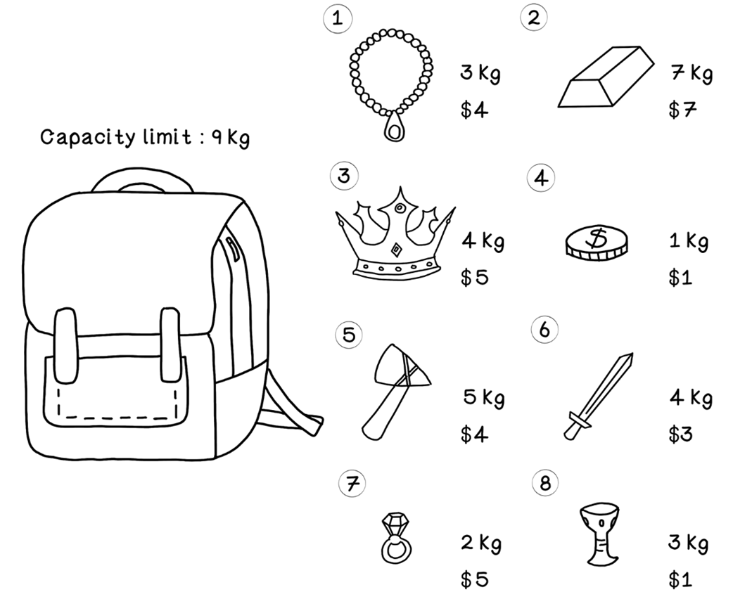
The example Knapsack Problem
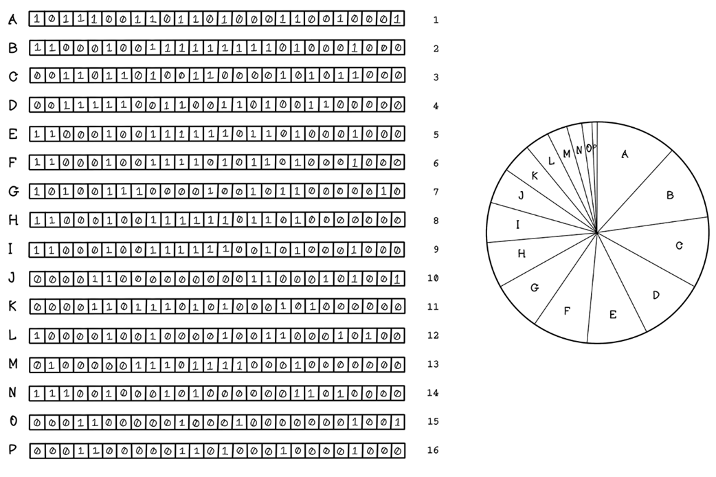
Example of rank selection
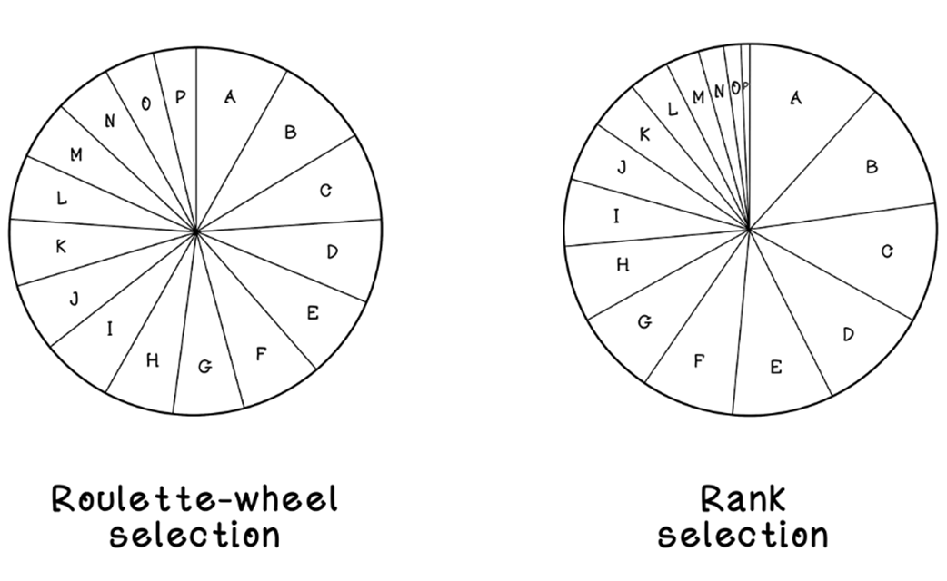
Roulette-wheel selection vs. rank selection
Example of tournament selection
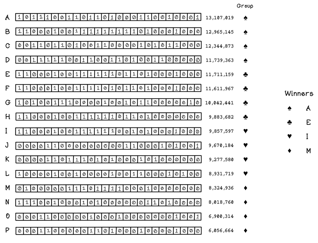
Example of elitism selection
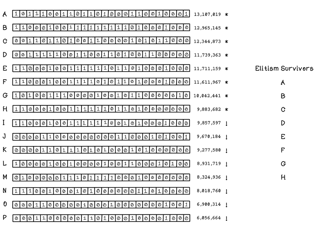
Example of real-value encoding
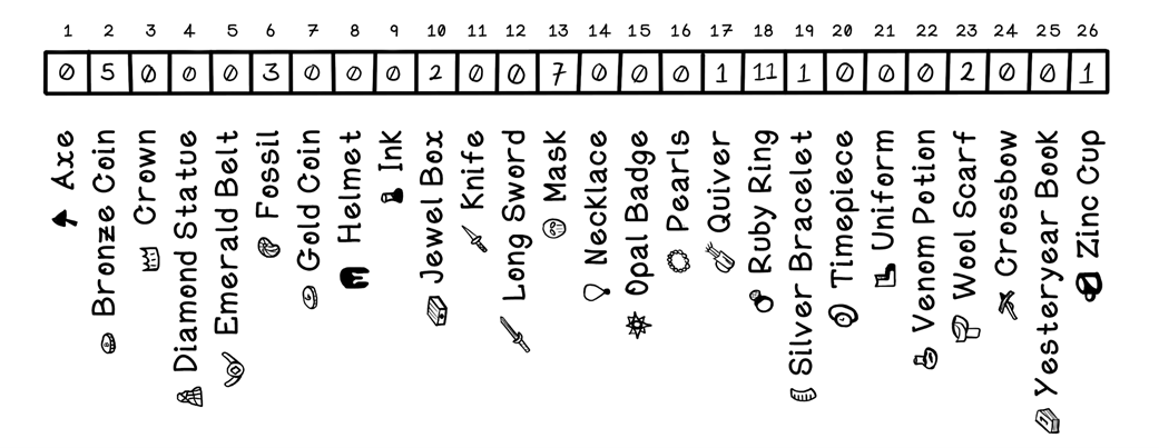
Example of arithmetic crossover
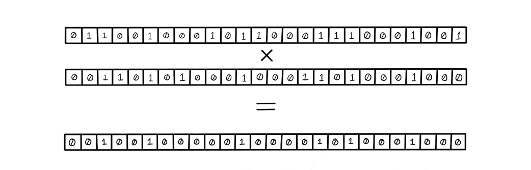
Example of boundary mutation
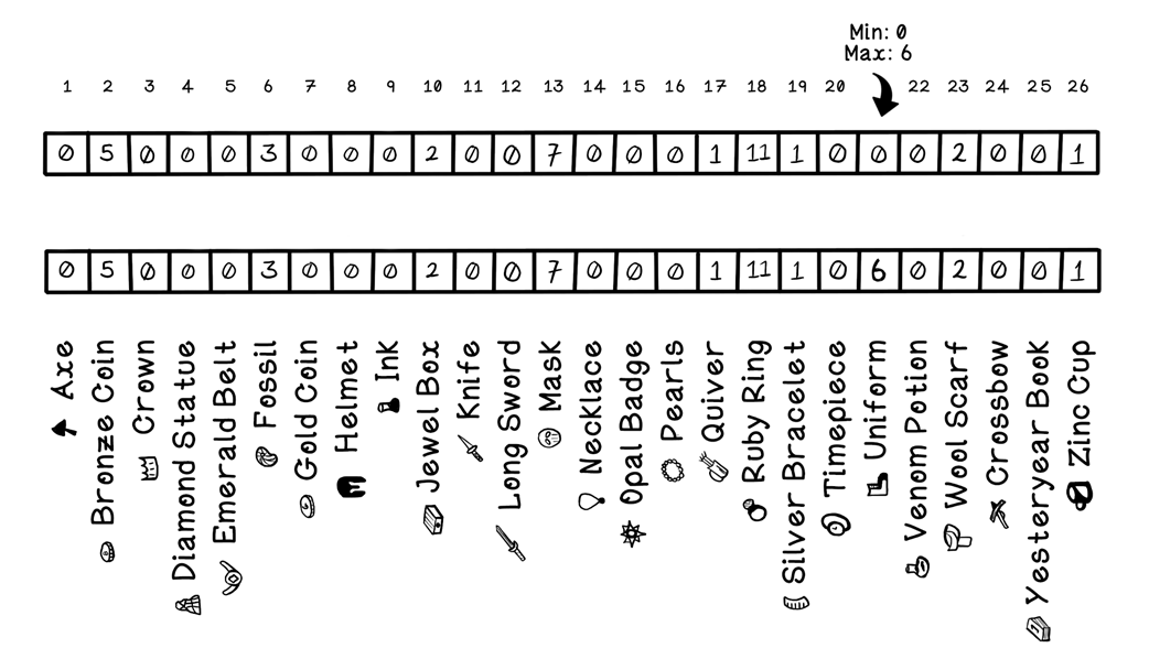
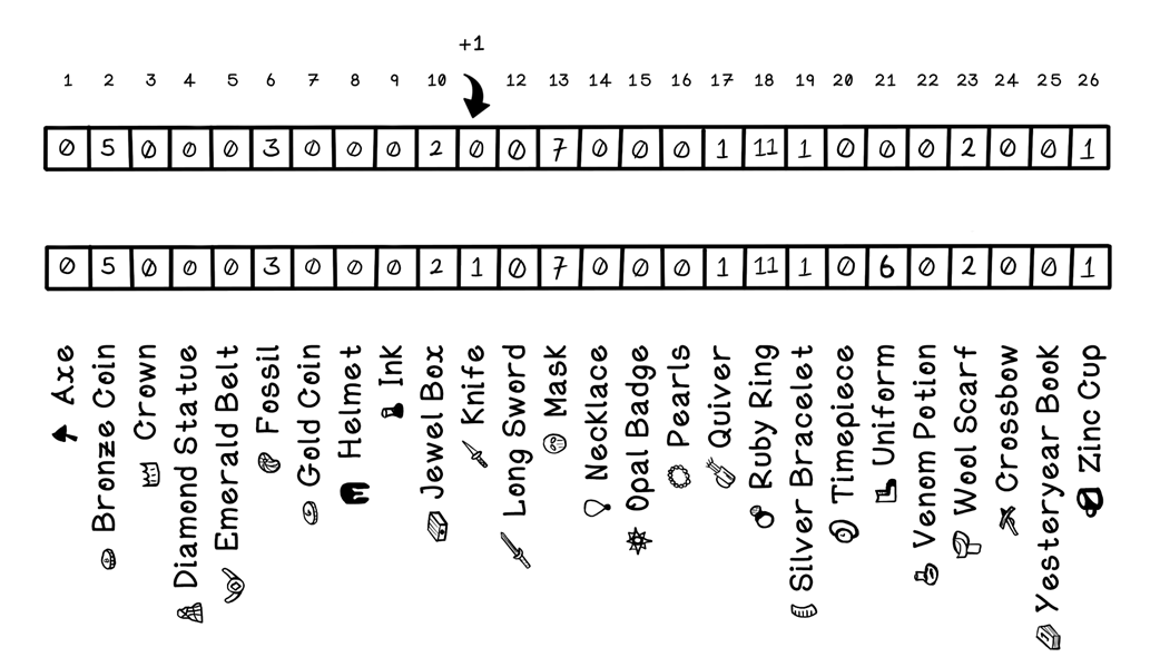
Example of arithmetic mutation
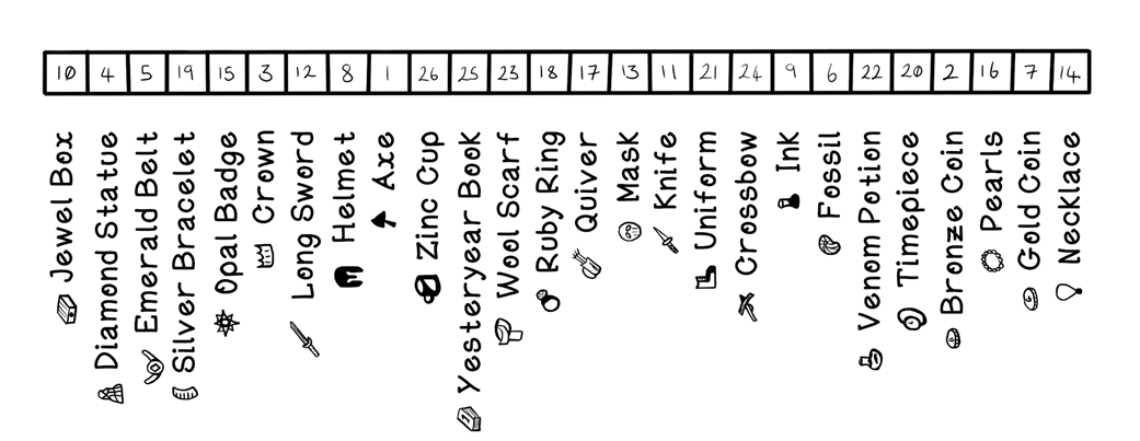
Example of order encoding
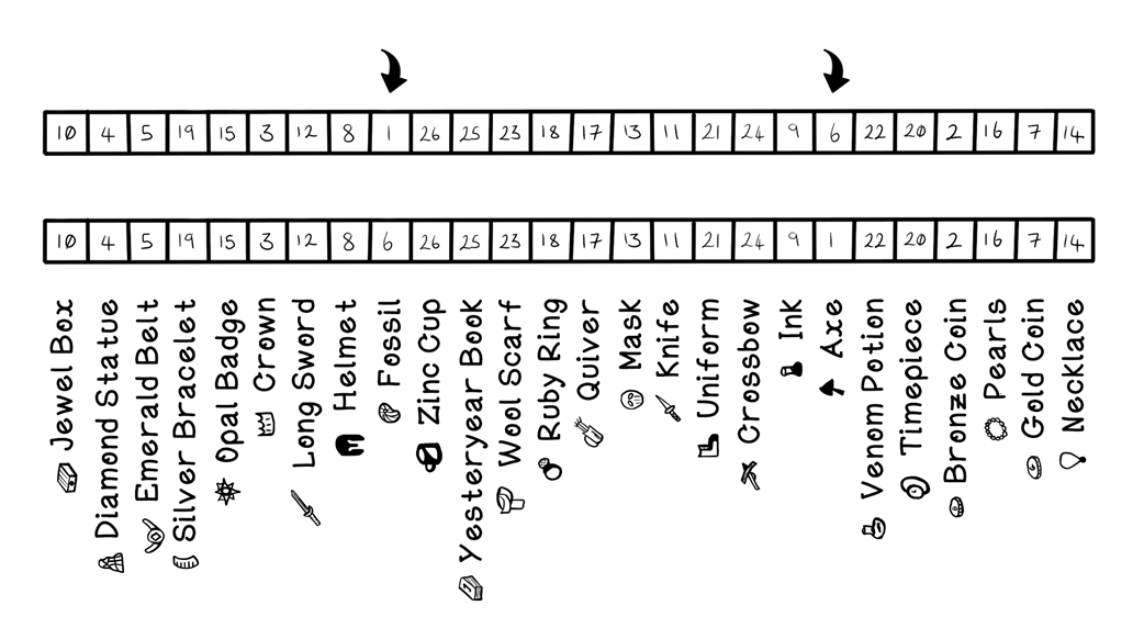
Example of order mutation
Example of a tree used to represent the Wagon Packing Problem
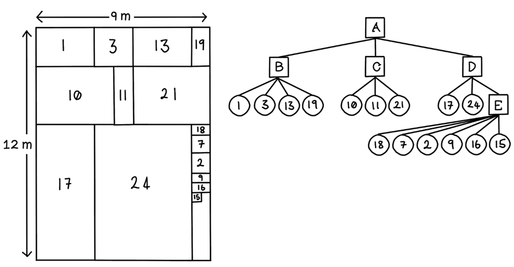
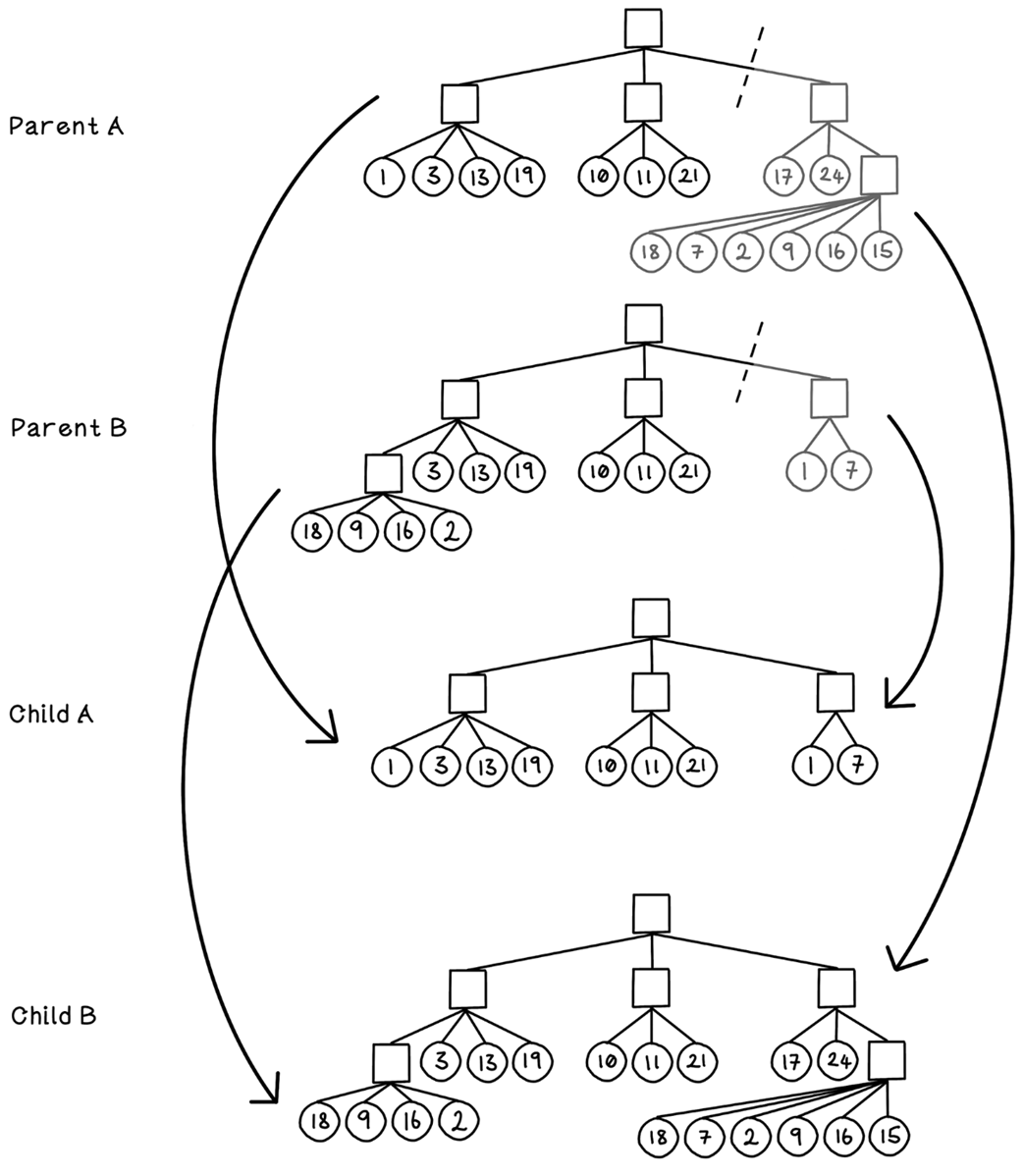
Example of tree crossover
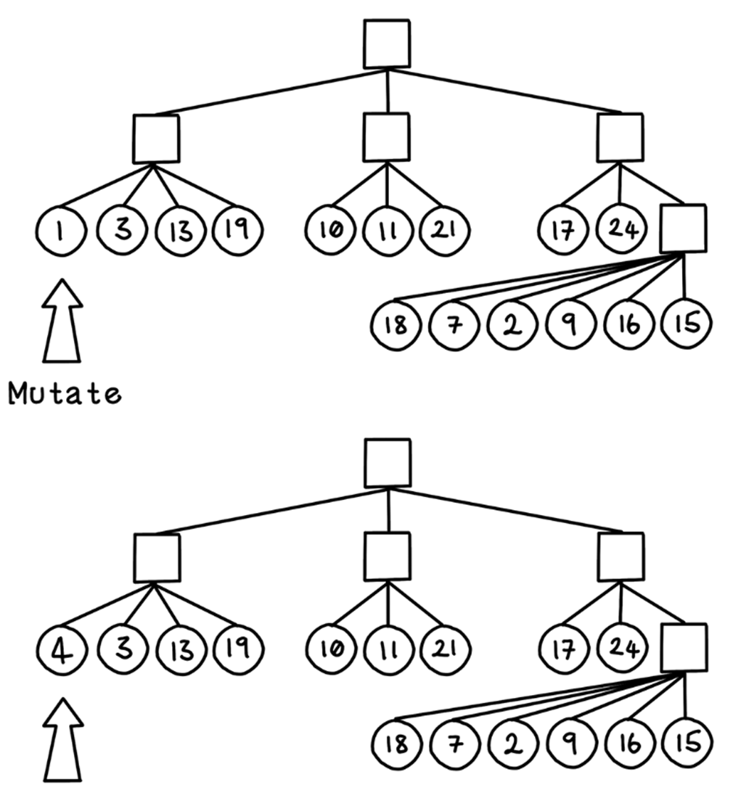
Change node mutation in a tree
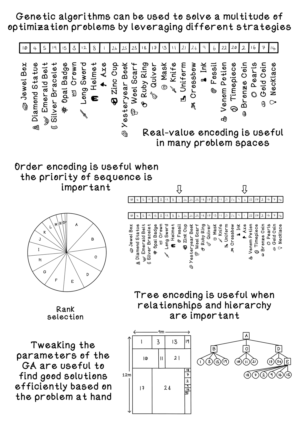
Summary of advanced evolutionary approaches
FAQ
How do I choose between binary, real-value, order, and tree encoding for a genetic algorithm?
- Binary: Select/ignore items (on/off decisions) like the basic Knapsack Problem.
- Real-value: Quantities or continuous parameters (e.g., multiple units, coordinates, weights).
- Order (permutation): Visit/process every item exactly once but sequence matters (scheduling, routing, refinery ordering).
- Tree: Hierarchical or compositional structures (packing layouts, program structures in genetic programming). Choose the encoding that most naturally matches the decision variables and constraints of your problem.
What are the key differences between rank selection, tournament selection, and elitism?
- Rank selection: Replaces raw fitness with ranks to reduce bias from large fitness gaps; improves fairness and diversity.
- Tournament selection: Picks the best from small random groups; easy to tune via group size; larger tournaments increase selection pressure but reduce diversity.
- Elitism: Copies top individuals directly to the next generation to avoid losing the best-so-far; too much elitism risks premature convergence.
How does tournament size influence selection pressure and population diversity?
- Small tournaments (size 2–3): Lower pressure, higher diversity, more exploration.
- Medium (size 4–6): Balanced exploration/exploitation for many problems.
- Large (size 7+): High pressure, faster convergence, higher risk of local optima. Adjust size with mutation rate and elitism to maintain a healthy search.
What is arithmetic crossover and why is it suited to real-value encoding?
Arithmetic crossover combines parent genes via operations (e.g., weighted sums, products) to produce numeric offspring. It’s ideal for continuous parameters because results stay meaningful without ad hoc rounding. Caution: simple averaging can pull children toward midpoints, which helps early exploration but may “wash out” precise peaks later; consider adaptive weights or mix with other operators.
When should I use boundary mutation versus arithmetic mutation with real-valued genes?
- Boundary mutation: Sets a chosen gene to its min or max. Use to test extremes, escape local optima, or when bounds have special meaning (e.g., “fill or skip”).
- Arithmetic mutation: Adds/subtracts a small delta. Use for fine-grained local search and continuous tuning. Many workflows alternate both to balance jumps and refinements.
Why can’t I use standard crossover with order (permutation) encoding, and what should I use instead?
Standard crossover often introduces duplicates or loses items, violating permutation constraints. Use permutation-safe operators such as PMX (Partially Mapped Crossover), OX (Order Crossover), or CX (Cycle Crossover), which preserve item uniqueness while shuffling order. Mutation typically swaps two positions to maintain validity.
Why is the fitness function especially critical in the Refinery (ordering) scenario?
Success depends on maintaining a minimum value rate over time, not just total value. The fitness must model sequence-dependent throughput using item values and extraction times. Tips: compute a time-profile of accumulated value per hour, penalize dips below the target rate, handle ties/edges consistently, and validate logic with simple, known sequences.
How does tree encoding solve the Wagon Packing Problem, and what do its operators look like?
Tree encoding represents recursive layout decisions (e.g., split horizontal vs vertical, then pack subsets). Tree crossover swaps subtrees between parents to inherit layout strategies; change-node mutation replaces a node (e.g., split type or assigned item/group) with another valid option. Always validate children against constraints (sizes, non-overlap, capacity).
What’s the difference between genetic programming and evolutionary programming, and where does neuroevolution fit?
- Genetic programming (GP): Evolves program structures (often trees) that directly solve tasks; outputs can be hard to interpret but flexible.
- Evolutionary programming (EP): Evolves parameter sets for an existing fixed program or model.
- Neuroevolution: A form of EP/EA applied to neural networks, evolving architectures and/or hyperparameters (and sometimes weights).
How do I balance exploration and exploitation in advanced evolutionary approaches?
- Increase exploration: Smaller tournaments, lower elitism, higher mutation rate, boundary mutations, larger populations.
- Increase exploitation: Larger tournaments, modest elitism (e.g., 1–5% of population), lower mutation with arithmetic/local tweaks, focused crossover.
- Practical tips: Start exploratory, then gradually raise selection pressure or lower mutation; monitor diversity and best-fitness plateaus; set clear stopping criteria (no-improvement window, budget, or target).

 Grokking AI Algorithms, Second Edition ebook for free
