Overview

2 Search fundamentals

This chapter introduces planning and searching as core behaviors of intelligent systems: we form plans, then adapt them as reality changes, using search to choose and revise the next best steps toward our goals. Search is framed as evaluating possible future states to reach a target efficiently, with an emphasis on why “smart” algorithms matter: computational cost grows quickly with naive exploration, so understanding Big O complexity and avoiding brute force is essential. The text also clarifies what kinds of problems fit search—any task requiring a sequence of decisions—illustrated with maze pathfinding, and stresses that good algorithms aim for optimal or at least high-quality solutions under real-world constraints.

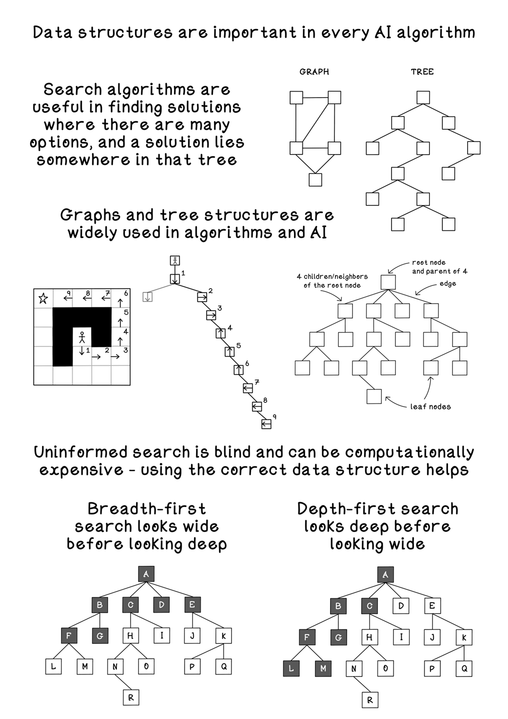
A major focus is representing problem spaces so computers can process them consistently and efficiently. The chapter distinguishes data (raw facts) from information (interpreted, contextualized facts), then surveys data structures that enable effective search. Graphs model states (nodes) and transitions (edges, possibly weighted), and can be encoded in several concrete forms (edge lists, matrices, adjacency lists) to support different performance needs. Trees—connected, acyclic structures—capture solution paths with concepts like root, parent/child, depth, height, leaves, and path cost. Rather than constructing the full tree of possibilities upfront, search algorithms generate and traverse these structures incrementally to keep computation tractable.

Two uninformed (“blind”) search strategies are developed. Breadth-first search uses a FIFO queue to expand all nodes at a given depth before moving deeper; on unweighted graphs it guarantees the shortest path but can be memory intensive. Depth-first search uses a LIFO stack to dive along one branch before backtracking; it is memory efficient but not guaranteed to find the shortest route. Both rely on tracking visited states to avoid cycles. The chapter closes with practical applications—network routing, web crawling, and social connectivity—and a brief tour of graph categories (directed/undirected, acyclic, complete, weighted) and representations, reinforcing how the choice of model and algorithm shapes efficiency and solution quality.

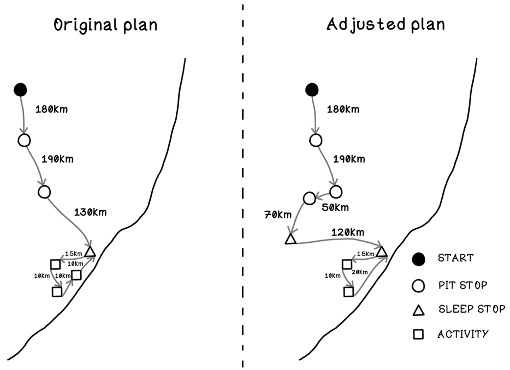
Example of how plans change in projects
Original plan versus adjusted plan for a road trip
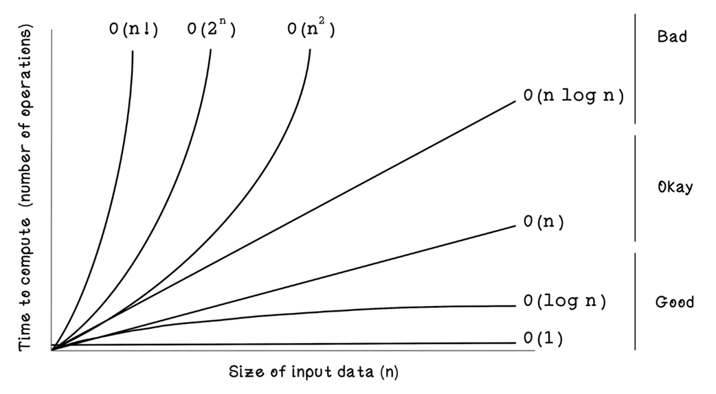
Big O complexity
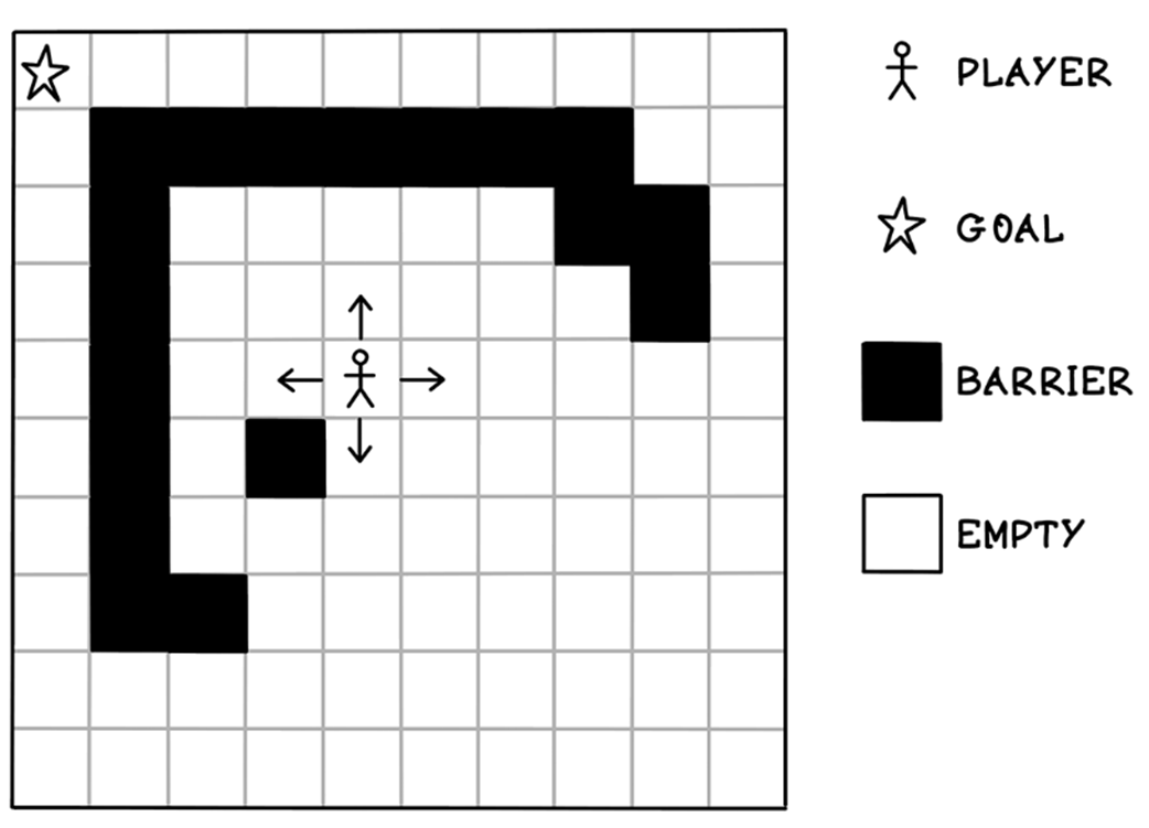
An example of the maze problem
Examples of possible paths to the maze problem
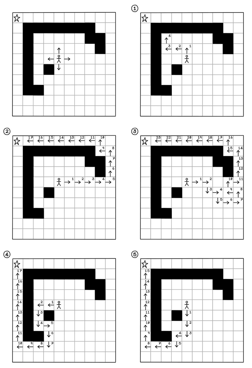
A large example of the maze problem

Data versus information
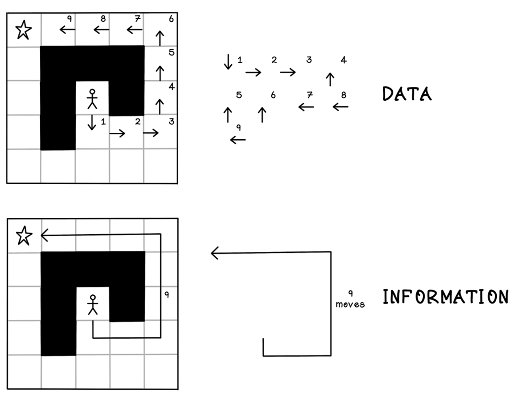
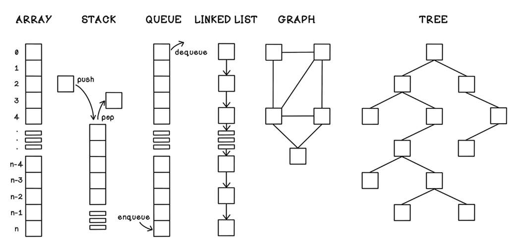
Data structures used with algorithms
The notation used to represent graphs
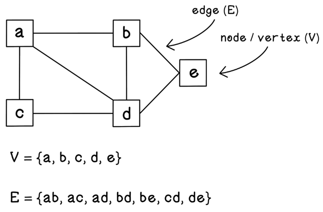
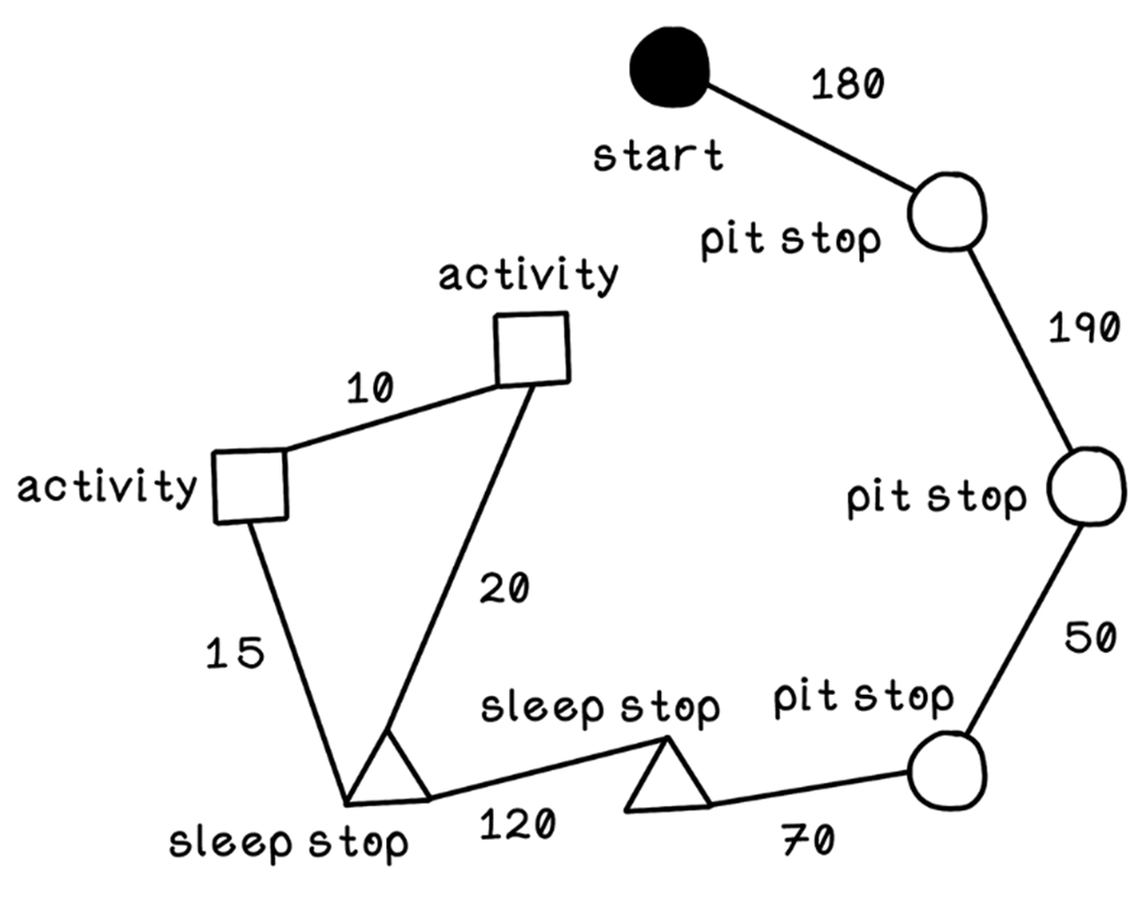
The example road trip represented as a graph
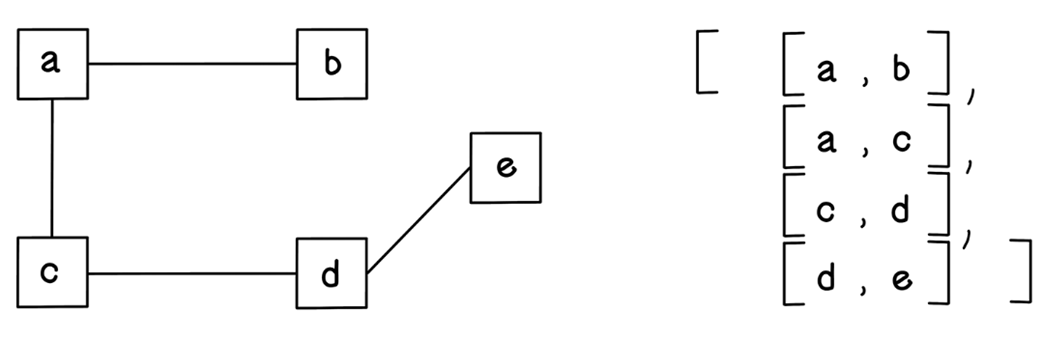
Representing a graph as an array of arrays
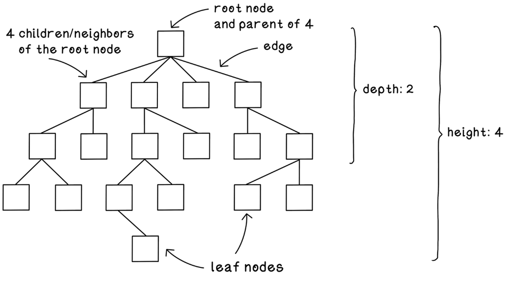
The main attributes of a tree
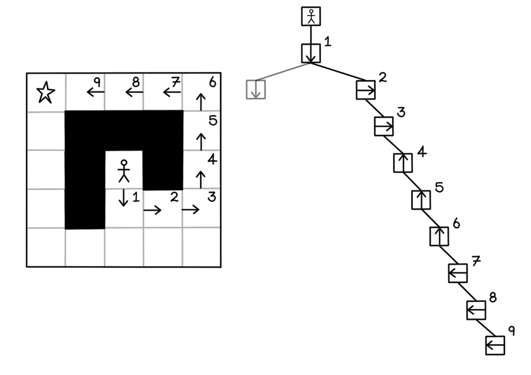
A solution to the maze problem represented as a tree
The constraint for the maze problem
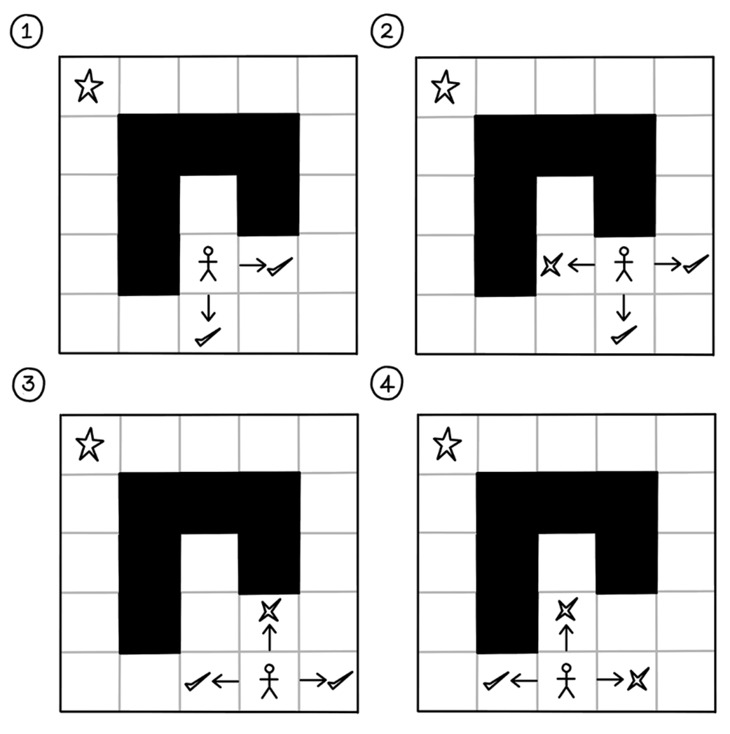
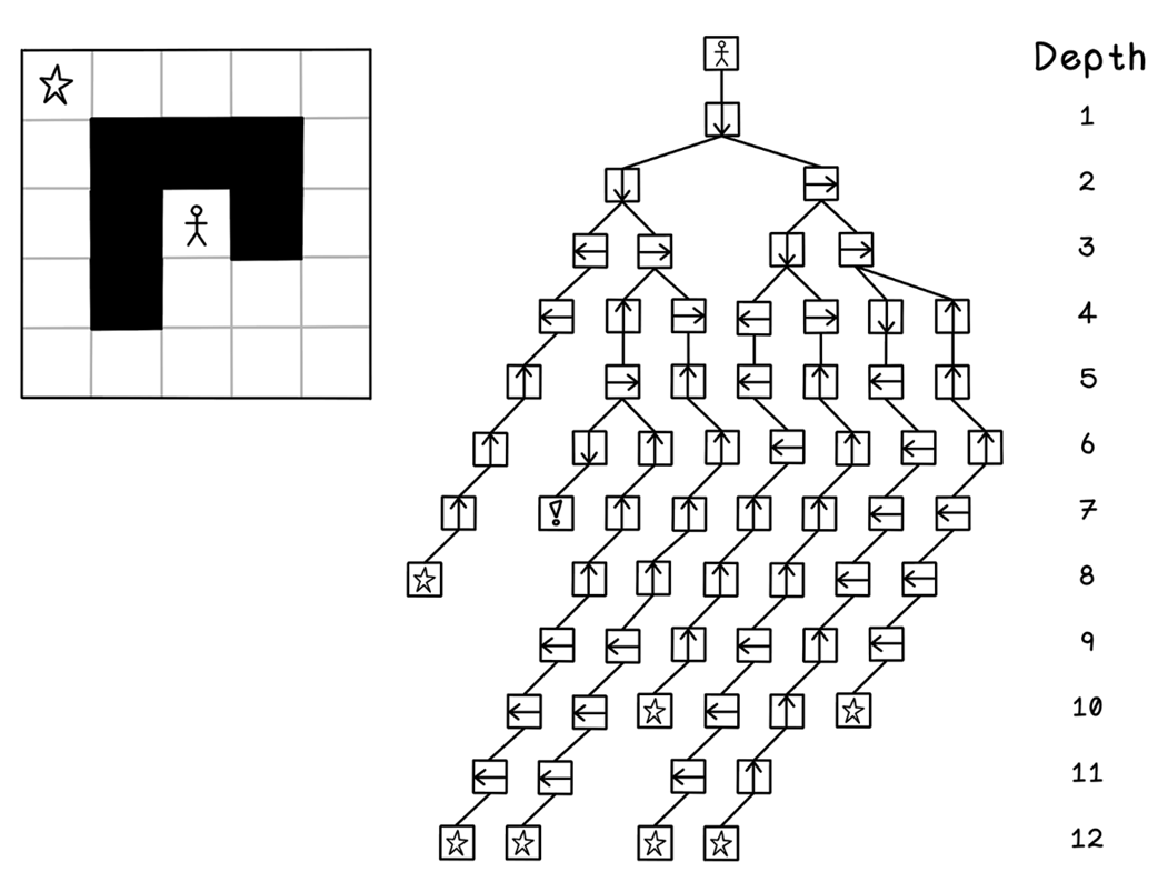
All possible movement options represented as a tree
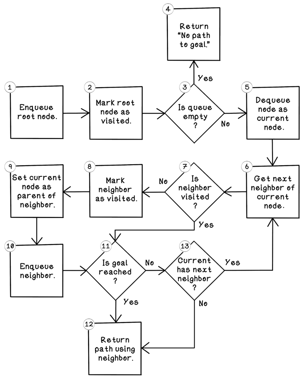
Flow of the breadth-first search algorithm
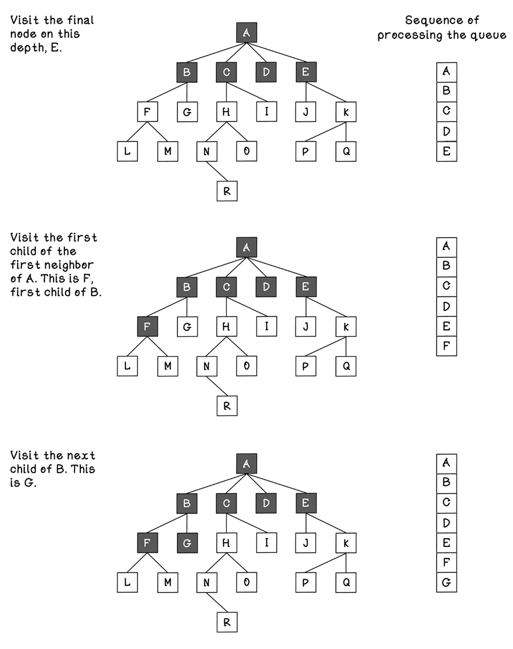
The sequence of tree processing using breadth-first search (part 1)
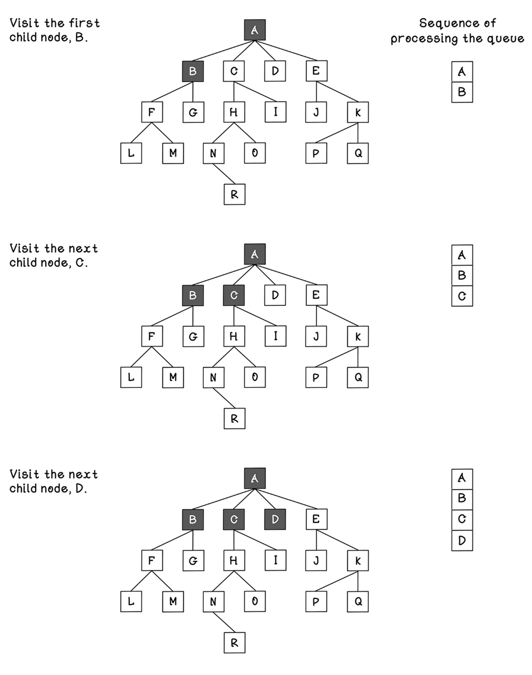
The sequence of tree processing using breadth-first search ( part 2)
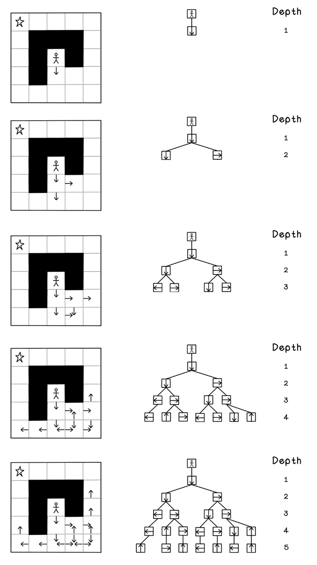
Maze movement tree generation using breadth-first search
Nodes visited in the entire tree after breadth-first search
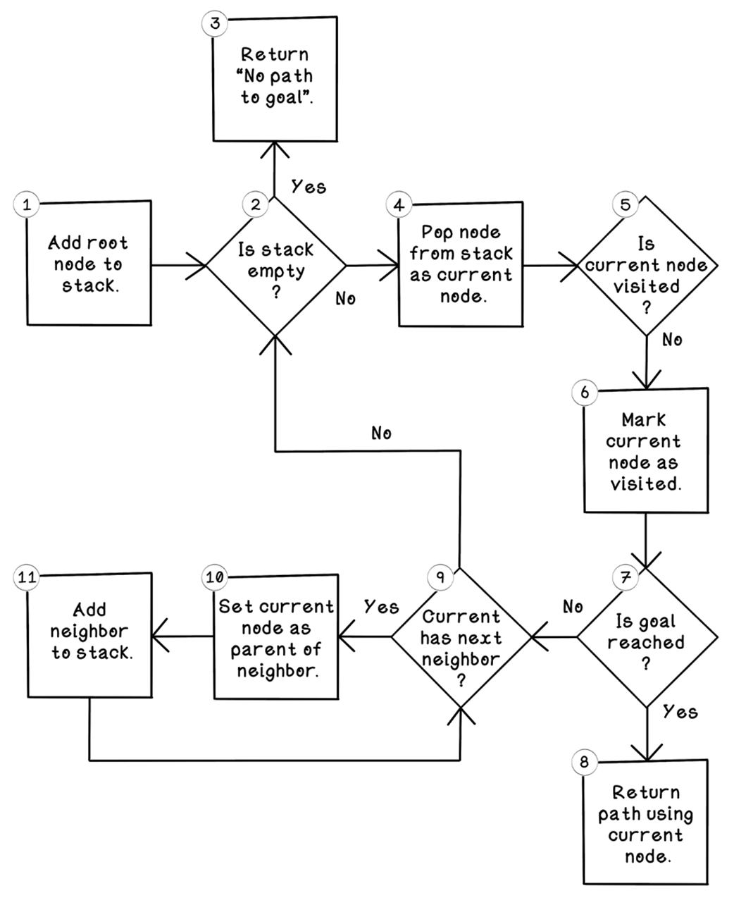
Flow of the depth-first search algorithm
The sequence of tree processing using depth-first search (part 1)
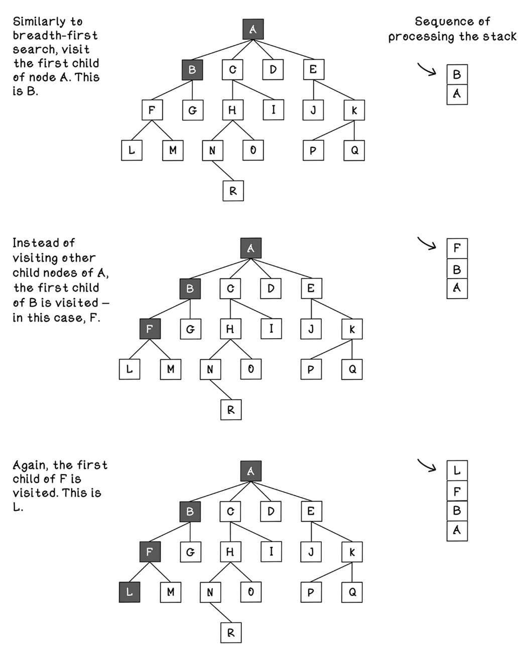
The sequence of tree processing using depth-first search (part 2)
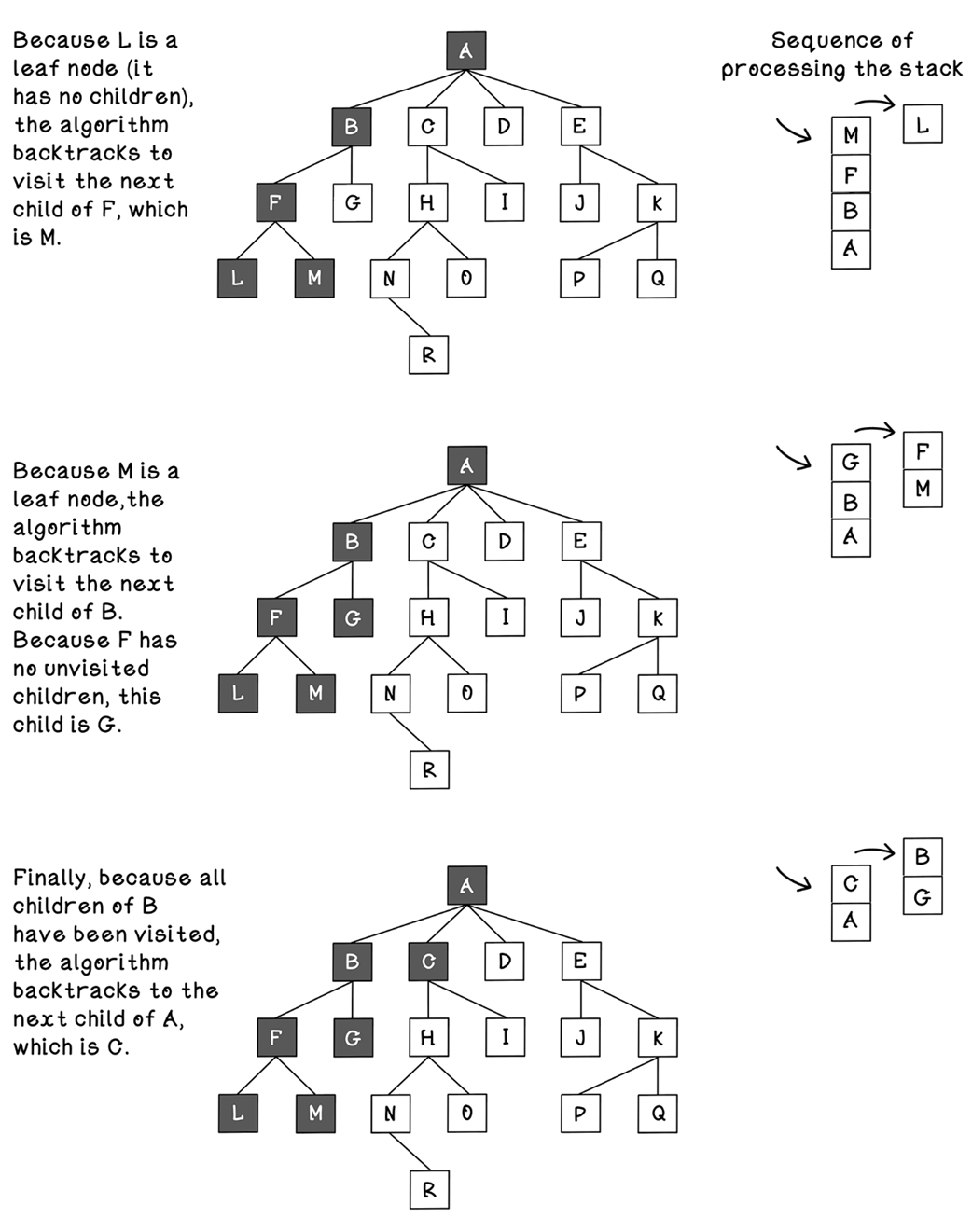
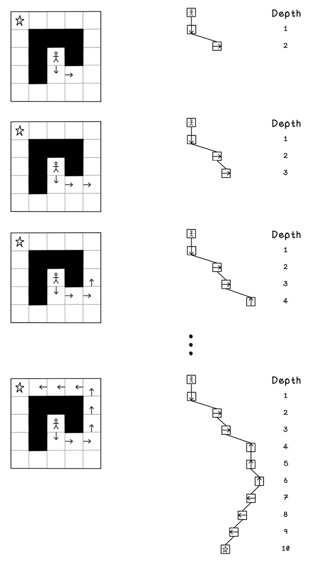
Maze movement tree generation using depth-first search
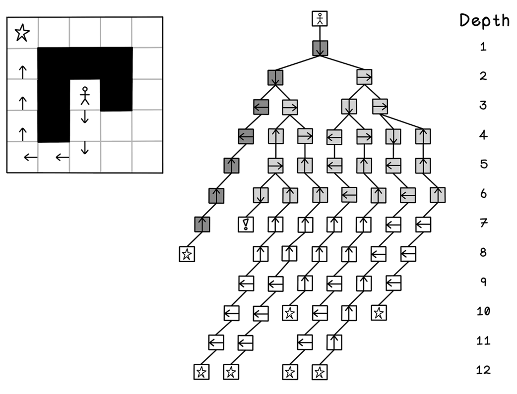
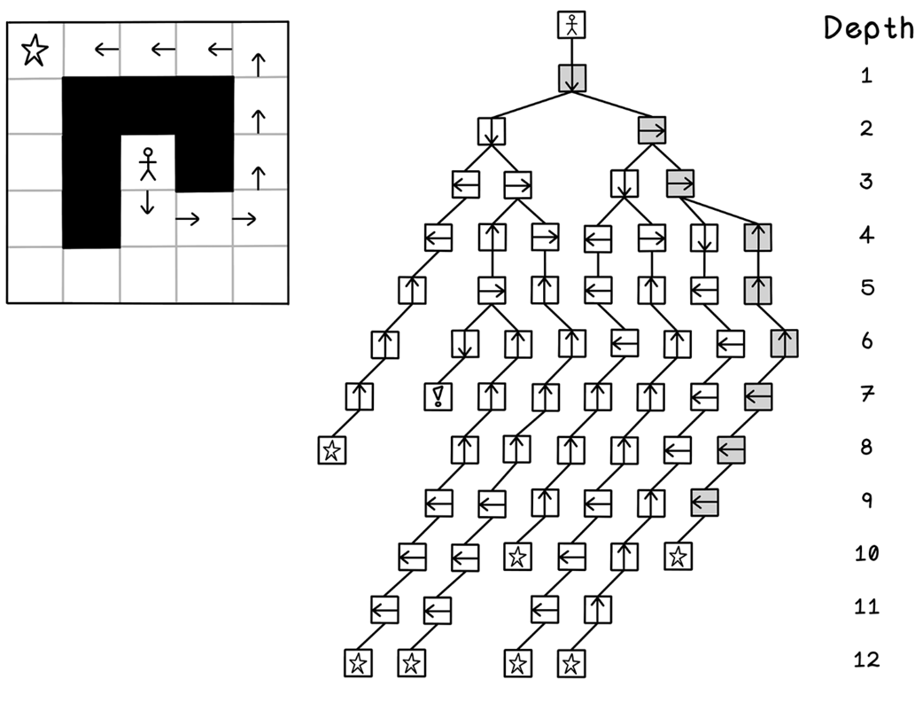
Nodes visited in the entire tree after depth-first search
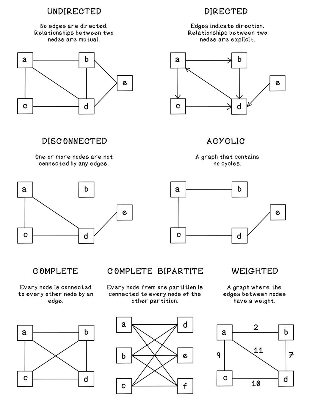
Types of graphs
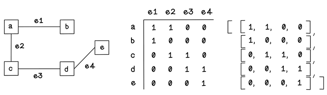
Representing a graph as an incidence matrix
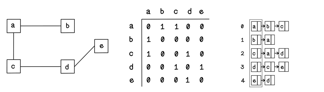
Representing a graph as an adjacency list
Summary of search fundamentals

FAQ

What’s the difference between planning and searching?Planning is deciding a sequence of actions to reach a goal, often updated as situations change. Searching is the mechanism that guides planning by exploring possible future states and selecting steps that move you closer to the goal.
Why does computation cost (Big O) matter for search algorithms?As problem size grows, the number of operations can explode. Big O notation helps estimate time and space needs so we choose algorithms and data structures that scale, avoiding brute force when it’s infeasible.
Which problems are well-suited to search algorithms?Any task requiring a sequence of decisions, such as finding shortest paths in mazes, routing in networks, scheduling, or puzzle solving. Depending on constraints, search may find the optimal answer or a good-enough solution.
How do we represent a problem so a search algorithm can process it?Model the problem as states and transitions—commonly a graph with nodes (states) and edges (actions). Encode data consistently (e.g., grids, coordinates, adjacency structures), and define start, goal, valid moves, and costs.
What’s the difference between graphs and trees in search?A graph captures all states and their connections (and may contain cycles). A search tree is the unfolding of explored paths from a start state, typically acyclic, used to trace and return a single solution path.
How does Breadth-First Search (BFS) work and when should I use it?BFS explores level by level using a FIFO queue, visiting all nodes at depth d before d+1. It guarantees the shortest path in unweighted graphs but can use lots of memory because it stores entire frontiers.
How does Depth-First Search (DFS) work and when should I use it?DFS dives along a path using a LIFO stack (or recursion) until a dead end, then backtracks. It uses little memory but doesn’t guarantee the shortest path; it returns the first solution it finds.
How do search algorithms avoid infinite loops or revisiting states?Maintain a visited set (or mark nodes) and, when building paths, avoid moving back to previously visited states. For graphs with cycles, this bookkeeping is essential to prevent catastrophic looping.
What real-world applications use uninformed search?- Network routing to connect devices across hops - Web crawling to follow links and index pages - Social graph queries (e.g., “friend-of-a-friend”) to suggest connections
What are common graph representations and categories I should know?- Representations: adjacency list, adjacency matrix, incidence matrix—choose based on sparsity, memory, and edge-centric needs. - Categories: directed/undirected, acyclic, disconnected, complete, weighted—these properties influence which search or optimization methods are appropriate.

pro $24.99 per month

  • access to all Manning books, MEAPs, liveVideos, liveProjects, and audiobooks!
  • choose one free eBook per month to keep
  • exclusive 50% discount on all purchases
  • renews monthly, pause or cancel renewal anytime

lite $19.99 per month

  • access to all Manning books, including MEAPs!

team

5, 10 or 20 seats+ for your team - learn more


choose your plan

team

monthly
annual
$49.99
$499.99
only $41.67 per month
  • five seats for your team
  • access to all Manning books, MEAPs, liveVideos, liveProjects, and audiobooks!
  • choose another free product every time you renew
  • choose twelve free products per year
  • exclusive 50% discount on all purchases
  • renews monthly, pause or cancel renewal anytime
  • renews annually, pause or cancel renewal anytime
  • Grokking AI Algorithms, Second Edition ebook for free

choose your plan

team

monthly
annual
$49.99
$499.99
only $41.67 per month
  • five seats for your team
  • access to all Manning books, MEAPs, liveVideos, liveProjects, and audiobooks!
  • choose another free product every time you renew
  • choose twelve free products per year
  • exclusive 50% discount on all purchases
  • renews monthly, pause or cancel renewal anytime
  • renews annually, pause or cancel renewal anytime
  • Grokking AI Algorithms, Second Edition ebook for free