15 Sampling continuous distributions

This chapter introduces the challenge of generating random samples from one-dimensional continuous distributions, extending ideas that were already used for categorical distributions. It explains that continuous distributions describe real-valued random processes with probability density functions, where probabilities are represented by areas under curves rather than by discrete weights. The chapter sets up the main goal: learning practical ways to simulate continuous random phenomena, especially when the distribution is known, partly known, or only available as a non-normalized density.

It first covers special-purpose sampling methods for common distributions, beginning with the continuous uniform distribution and then the normal distribution. The uniform case is straightforward because values can be drawn directly from a range, while the normal distribution is generated efficiently with the Box-Muller transform, producing bell-shaped samples centered around a mean with a chosen spread. The chapter also shows how histograms can be used to visualize sampled data and confirm that the generated values match the expected distribution.

Next, the chapter explains the inverse transform method, which samples from any continuous distribution as long as its cumulative distribution function or quantile function is known. This is illustrated with the Cauchy distribution, showing how a PDF, CDF, and inverse CDF work together to enable compact sampling code. Finally, it presents rejection sampling as a more general technique for sampling from distributions that are hard to sample directly, including clamping unwanted tails to a limited range; it also emphasizes the method’s drawbacks, especially inefficiency and the need for manual choice of a suitable helper distribution and scaling factor.

A PDF is like a probability mass function but defined over a range of real numbers rather than over discrete items. To sample, uniformly choose a point in the shaded area; the x coordinate of that point is the sample value.

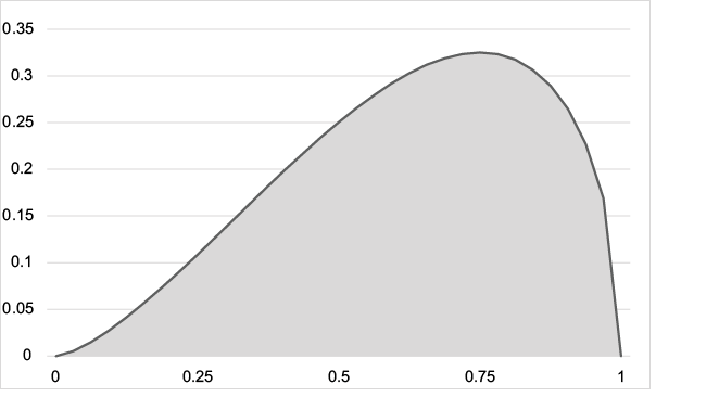
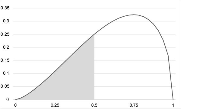
The probability that a sample from this distribution is less than 0.5 is proportional to the shaded area and equal to that shaded area divided by the shaded area in figure 15.1.

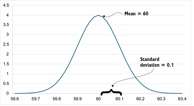
The PDF of a normal distribution with mean = 60.0 mm and standard deviation = 0.1 mm. This graph shows the normalized PDF; the area below the curve is 1.0.

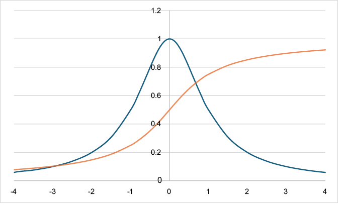
The normalized PDF and CDF of the standard Cauchy distribution. This distribution is useful when samples from the tails are more common than they are in a normal distribution. Almost all CDFs have a stretched S shape, called a sigmoid.

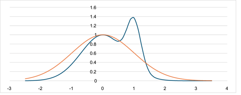
The two-hump function is the PDF of the desired distribution, and the one-hump function is the non-normalized standard normal distribution from section 15.3 that we’ll use as a helper. The helper’s PDF clearly isn’t larger than the target’s PDF everywhere, but we can fix that.

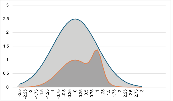
The target PDF is always smaller than the scaled-up helper PDF, so we can use rejection sampling. If we throw a dart, and it lands in the dark gray area, the x coordinate of the dart is the sample. If the dart lands in the light-gray area, we reject the throw and try again.

• A continuous probability distribution can be characterized by its PDF. A sample from a distribution is like throwing a dart uniformly at the area below the PDF and using its x coordinate as the sample. If the area below the PDF is 1.0, it’s said to be normalized. We frequently encounter non-normalized PDFs.
• The continuous uniform distribution generates random samples that are equally likely over a given range. If the range is 0.0 to 1.0, that’s the standard uniform distribution.
• The normal distribution describes a random process in which values deviate from a central value, the mean; this is the classic bell-shaped curve.
• The integral of a PDF is the CDF, the function which gives the probability that a sample will be less than a given value.
• The inverse of the CDF is the quantile function. We can sample from any distribution if we know its quantile function. Calling which function with a standard uniform sample generates a sample from the target distribution.
• If we don’t know the quantile function but have the PDF of a target distribution, sometimes we can find a helper distribution that allows us to use the rejection-­sampling algorithm. Finding a suitable helper distribution isn’t easy to automate, and arbitrarily many samples can be rejected before one is accepted.

FAQ