This chapter tackles interpretability for convolutional neural networks and shows that, unlike the “black box” stereotype, convnets learn visual concepts that can be made visible. It motivates interpretation for high-stakes domains and introduces three practical, complementary techniques: inspecting intermediate activations to see how inputs are decomposed, synthesizing filter visualizations to reveal what patterns filters respond to, and generating class-activation heatmaps to highlight image regions driving a decision. The chapter uses a small dogs-versus-cats model for activation inspection and a pretrained Xception network for filter visualization and class-localization examples.
Visualizing intermediate activations involves building a multi-output model that returns the outputs of convolution and pooling layers for a given image, then plotting each channel as a 2D map. The resulting grids reveal a progression: early layers behave like diverse edge/color detectors and retain much of the input detail; deeper layers become sparser and more abstract, encoding parts such as “cat ear/eye,” thereby distilling task-relevant information while discarding specifics—a hallmark of deep representations and analogous to human perception. Filter visualization uses gradient ascent in input space: define a loss as the mean activation of a target filter channel in a chosen layer, compute gradients, normalize updates, and iteratively adjust a random image to maximize that filter’s response. Implemented across TensorFlow, PyTorch, and JAX, the synthesized patterns evolve from simple edges and colors in shallow layers to compound textures and natural-image motifs higher up; a simple deprocessing step turns tensors into displayable images.
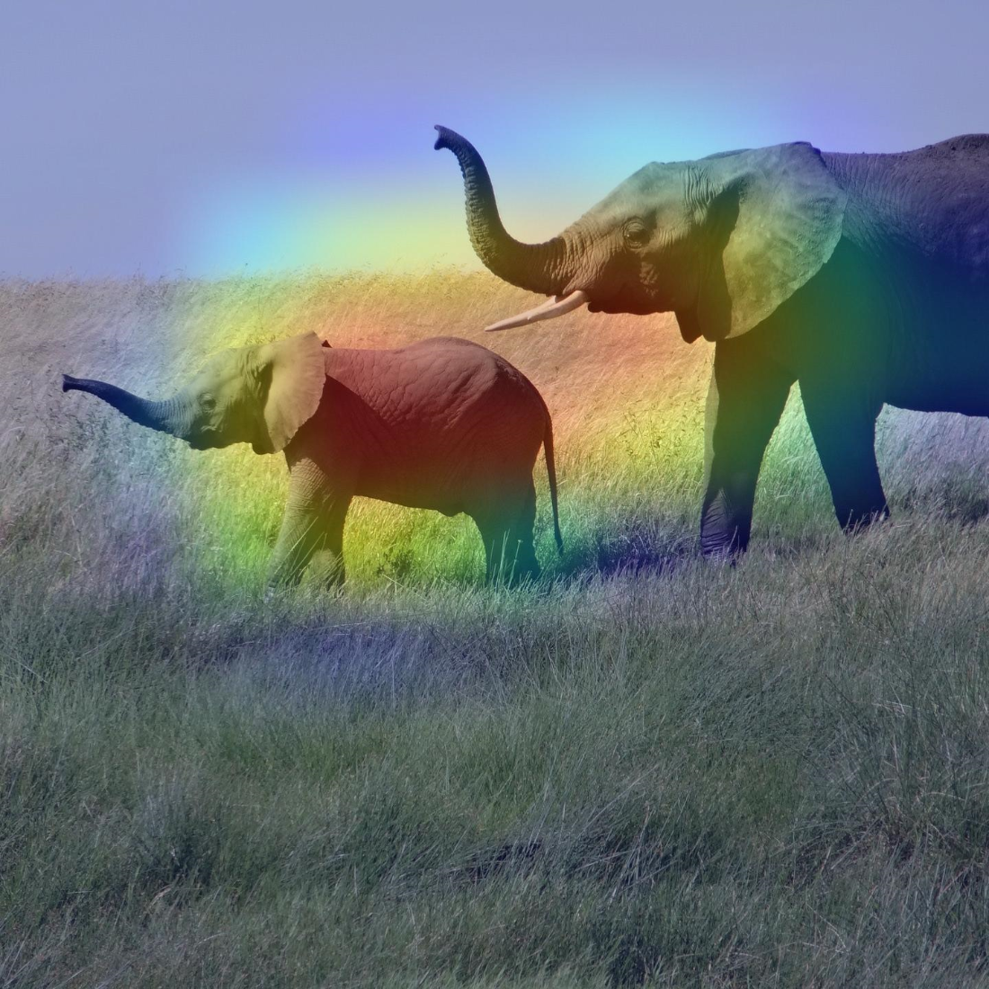
Class activation mapping (Grad-CAM) explains decisions and enables weak object localization by highlighting where the network “looked.” The method computes the last convolutional feature map for an input, obtains gradients of the target class score with respect to this map, globally averages these gradients to get channel-importance weights, and forms a heatmap by weighting and summing the channels, then normalizing and superimposing on the original image. Applied to an elephant photo with Xception, the heatmap emphasizes discriminative regions (for instance, ear shapes), answering both “why this class?” and “where is it?” in the image. Throughout, the chapter stresses correct preprocessing, the need to use differentiable model calls (model(x) vs. predict) when computing gradients, and the value of these tools for debugging, trust, and insight into convnet behavior.
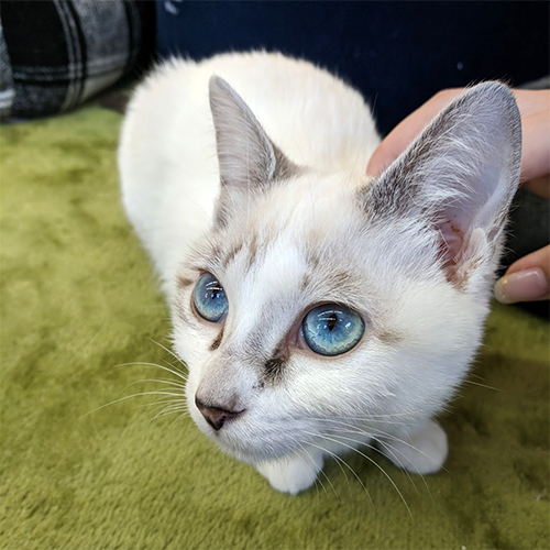
The test cat picture
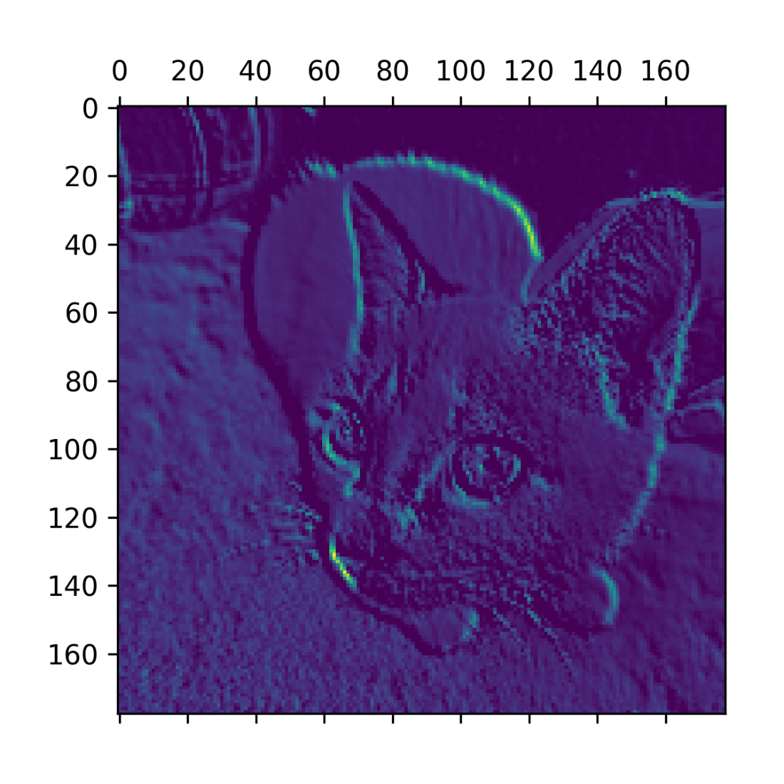
Sixth channel of the activation of the first layer on the test cat picture
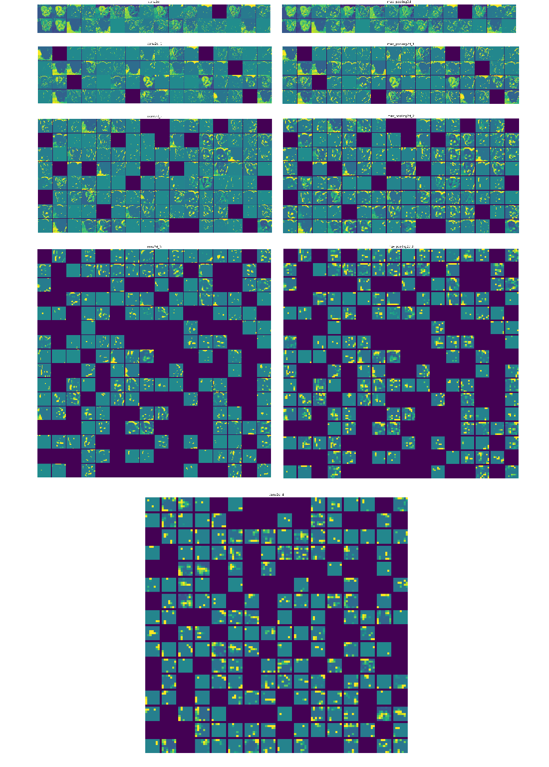
Every channel of every layer activation on the test cat picture
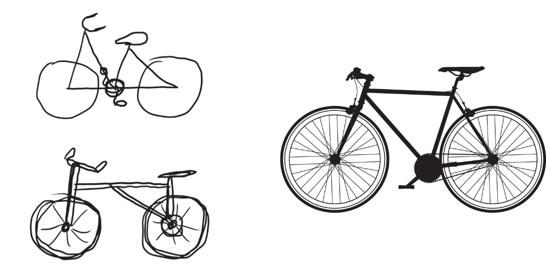
Left: attempts to draw a bicycle from memory. Right: what a schematic bicycle should look like.
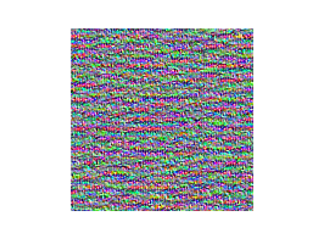
Pattern that the 2nd channel in layer block3_sepconv1 responds to maximally
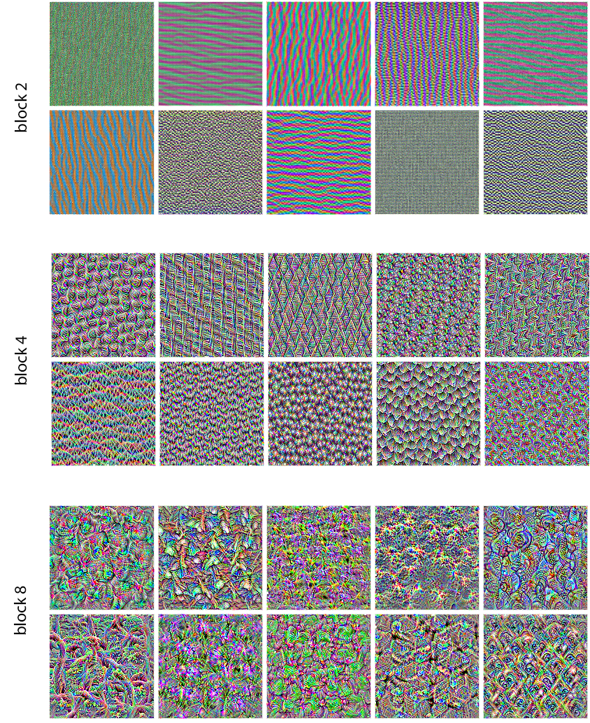
Some filter patterns for layers block2_sepconv1, block4_sepconv1, and block8_sepconv1.
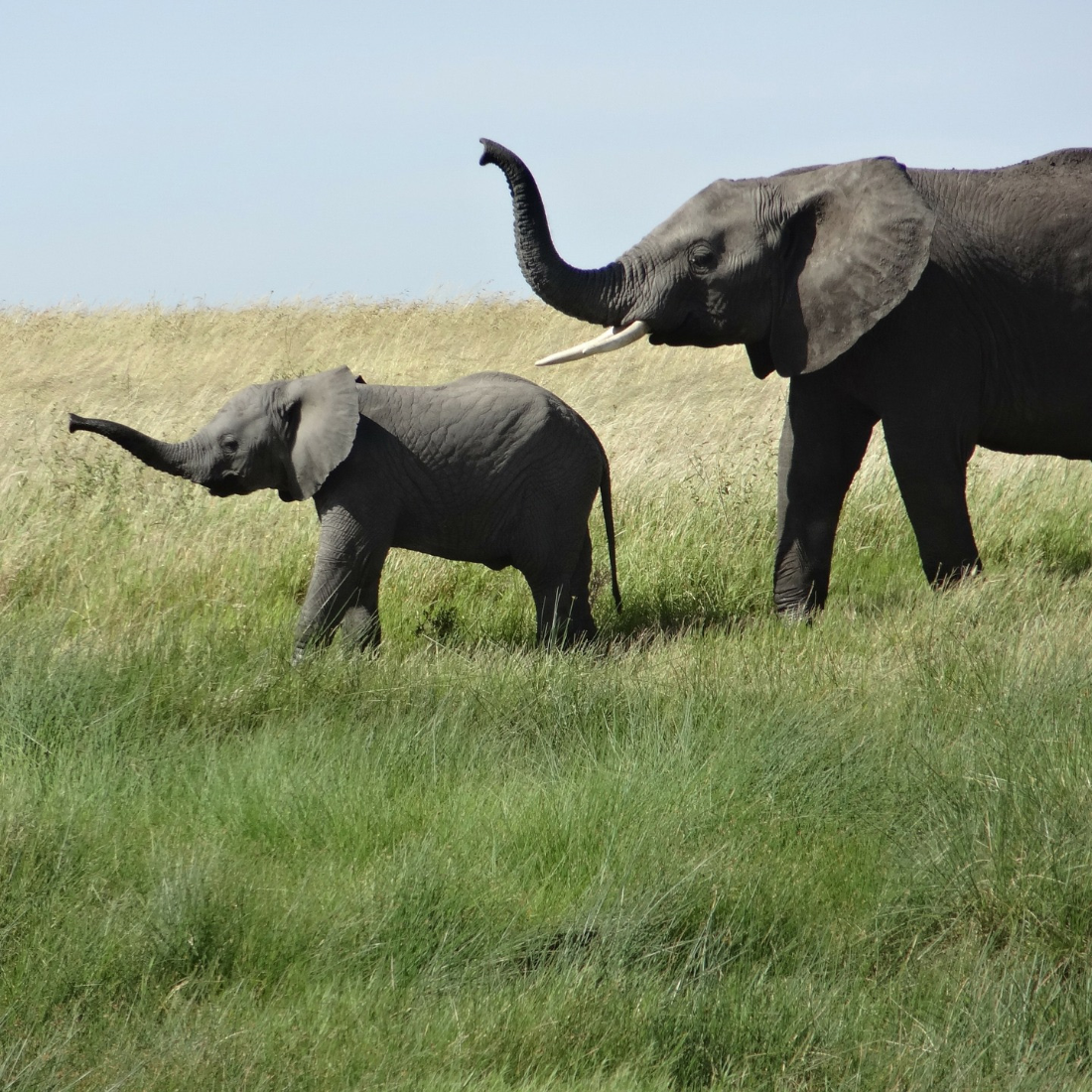
Test picture of African elephants
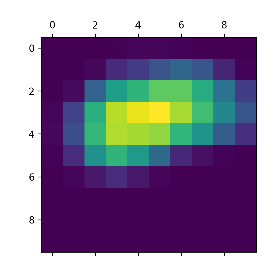
Standalone class activation heatmap.
African elephant class activation heatmap over the test picture
Chapter summary
Convnets process images by applying a set of learned filters. Filters from earlier layers detect edges and basic textures, while filters from later layers detect increasingly abstract concepts.
You can visualize both the pattern that a filter detects, and a filter’s response map across an image.
You can use the Grad-CAM technique to visualize what area(s) in an image were responsible for a classifier’s decision.
Together, these techniques make convnets highly interpretable.
FAQ
What does “interpreting what convnets learn” mean, and why does it matter?It refers to understanding how a convolutional neural network decomposes an image and what cues it uses to make predictions. Interpretation helps you trust, debug, and improve models, especially in sensitive domains like medical imaging, by revealing which visual concepts and regions drive decisions.Which visualization techniques are introduced in this chapter?The chapter focuses on three practical tools:
- Visualizing intermediate activations: shows how layers transform inputs and what each channel detects.
- Visualizing filters: uses gradient ascent to synthesize the pattern that maximally activates a chosen filter.
- Class activation maps (Grad-CAM): highlights image regions most responsible for a specific class prediction.How do I visualize intermediate activations for a given input image?Typical steps:
- Load a trained model and a test image, preprocess it to the model’s expected size and scale.
- Build a Keras model that takes the original input and outputs the activations of Conv2D/MaxPooling2D layers.
- Run a forward pass on the image to get a list of activation tensors.
- For each activation, plot individual channels as 2D images and arrange them in a grid to see what each filter responded to.What insights do intermediate activations reveal as depth increases?Common patterns:
- Early layers: edge and color detectors; most channels are active and preserve low-level details.
- Middle layers: simple textures and motif combinations.
- Deeper layers: abstract parts and class-specific cues (e.g., “eye,” “ear”); activations become sparser.
Overall, the network acts as an information distillation pipeline, discarding irrelevant detail and amplifying class-relevant signals.How can I visualize the pattern a specific convnet filter responds to?Use gradient ascent in input space:
- Select a target conv layer and filter index; create a feature-extractor model that outputs that layer.
- Define a loss as the mean activation of the target filter (crop borders to reduce artifacts).
- Initialize an input image with small random values; iteratively update it by ascending the gradient of the loss w.r.t. the input.
- Post-process the result (normalize, clip, optionally crop) to display the synthesized pattern.What backend differences exist for gradient ascent (TensorFlow, PyTorch, JAX)?All compute gradients but via different APIs:
- TensorFlow: use GradientTape to watch the input and get tape.gradient(loss, image); optionally @tf.function for speed.
- PyTorch: enable requires_grad on the input tensor, call loss.backward(), then read image.grad.
- JAX: define a loss function and use jax.grad(loss_fn) to obtain gradients; optionally jit for speed.What is Grad-CAM and how do I compute a class activation heatmap?Grad-CAM weights channels of a chosen conv layer by the gradient of the target class score:
- Build a model to get the last conv layer’s output, and another to map that output to final class scores.
- Compute the gradient of the desired class score w.r.t. the last conv feature map.
- Spatially average gradients over width and height to get per-channel importance weights.
- Weight the feature map channels by these weights, average across channels, apply ReLU, and normalize to [0,1] to obtain the heatmap.How do I overlay a Grad-CAM heatmap on the original image?Procedure:
- Rescale the heatmap to 0–255 and colorize it with a colormap (e.g., “jet”).
- Resize the colored heatmap to the original image size.
- Blend it with the original image (e.g., 40% heatmap + 60% image) and save or display the composite.When should I use model(x) vs model.predict(x) in these workflows?Use model.predict(x) to get outputs efficiently for large arrays; it’s non-differentiable and runs in batches. Use model(x) when you need gradients (e.g., gradient ascent, Grad-CAM), because autodiff frameworks can backpropagate through model(x) but not through predict().What practical tips and pitfalls should I watch for when interpreting convnets?Tips:
- Always match preprocessing to the pretrained backbone (size, scaling).
- Choose a meaningful conv layer: early for fine details, late for semantics (Grad-CAM usually uses the last conv).
- Normalize gradients during ascent to stabilize updates; watch learning rate and iterations.
- Expect non-determinism: filter visualizations vary between runs/seeds.
- Handle borders (cropping) to reduce artifacts; remember heatmaps are low-resolution and approximate.
- Don’t over-interpret single channels; look for consistent patterns across layers and inputs.
pro $24.99 per month
access to all Manning books, MEAPs, liveVideos, liveProjects, and audiobooks!
 Deep Learning with Python, Third Edition ebook for free