3 Single-qubit state and gates

This chapter introduces the single-qubit state as a pair of complex amplitudes that encode both probability (via squared magnitudes) and direction/phase. It presents a practical mental model and visualization called a state table, which lists outcomes, amplitudes, magnitudes, directions, and probabilities, and explains how phases influence computation even when probabilities stay the same. The chapter shows how to represent states in Python as lists of complex numbers, enforce normalization, compute magnitude and phase, and build a minimal simulator scaffold to initialize and inspect states.

The chapter then develops single-qubit gates and their effects, framing rotations as multiplication by a unit-magnitude complex number and highlighting the X, Z, Phase P(φ), Hadamard H, RZ(θ), and Y gates, followed by the RX and RY rotation families. It emphasizes that these are linear, unitary transformations that can be written as 2×2 matrices, have inverses (adjoints), and preserve total probability. A compact Python implementation encodes gates as nested lists and applies them with a generic transform that recombines amplitudes; circuits are built by sequencing such gates, with utilities to print and visualize the resulting states.

Finally, the chapter explains measurement as probabilistic sampling of outcomes according to the state’s distribution and shows how to simulate this with classical random sampling, where empirical frequencies converge to theoretical probabilities with more shots. It demonstrates practical single-qubit applications: preparing the uniform distribution (e.g., with H or π/2 rotations), encoding any Bernoulli distribution using RY with an angle chosen from p, and encoding real numbers either in an amplitude’s magnitude (via RY) or in an amplitude’s phase (via H followed by a Phase rotation). While a single qubit does not deliver quantum speedups, it is a useful vehicle for controlled sampling, data encoding, and for building intuition and tooling that generalize to multi-qubit systems.

Concepts introduced in this chapter.

Table 3.1 A single-qubit state has two possible outcomes.

Table 3.2 A single-qubit state has two amplitudes, each corresponding to a possible outcome.

A "clock" representation of a quantum state and the unit color wheel.

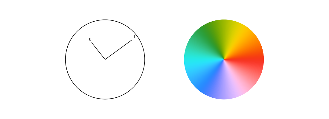
Table 3.3 A single-qubit state has two amplitudes. Each amplitude has a magnitude and direction.

Table 3.4 The probability of each outcome is the squared magnitude of the corresponding amplitude.

Table 3.5 The general form of a single-qubit state.

Table 3.6 The general form of a single-qubit state with amplitudes in polar form.

Table 3.7 The general form of a single-qubit state with amplitudes in polar form.

Table 3.8 The expanded state table for the example state encoded in Python above.

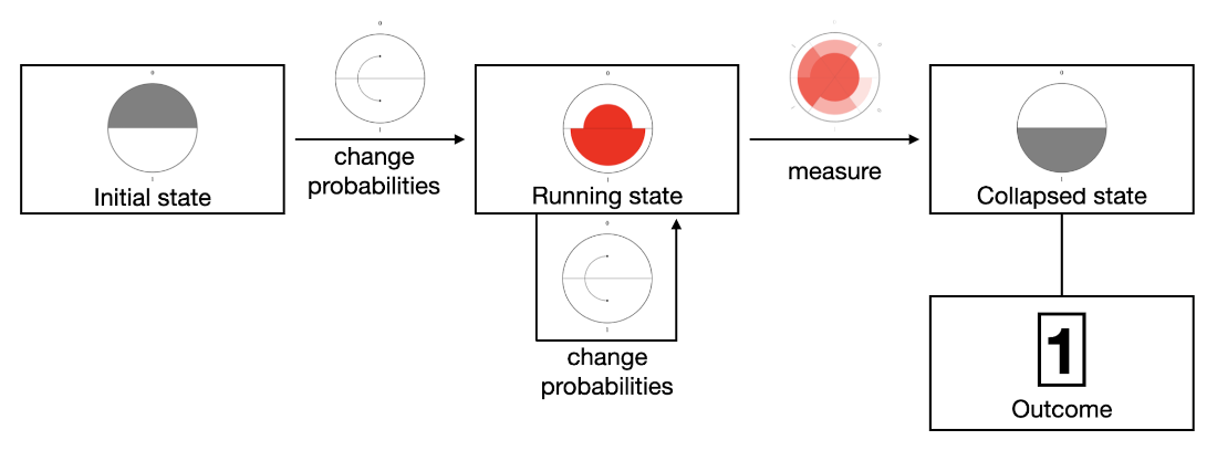
The steps of a single-qubit quantum computation.

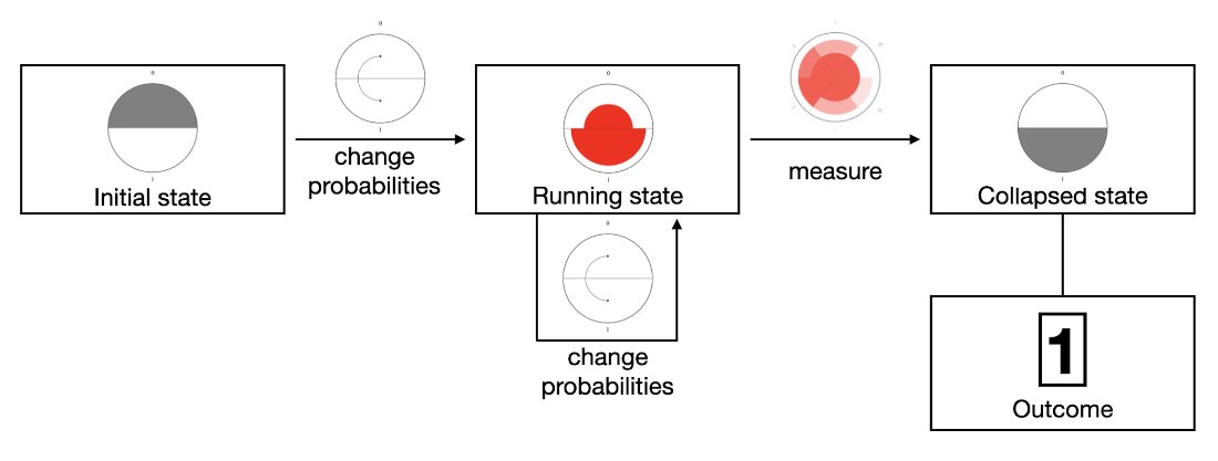
The effect of the X-gate on a pair of amplitudes

The effect of the X-gate on an example pair of amplitudes.

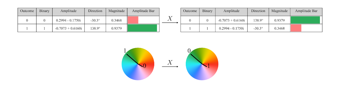
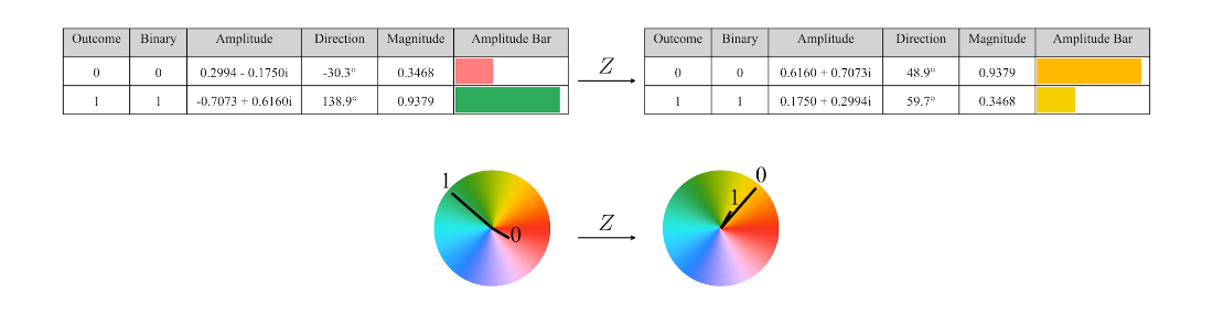
The effect of the Z-gate on a pair of amplitudes.

The effect of the Z-gate on a pair of probabilities with direction

The effect of the Z-gate on an example a pair of amplitudes.

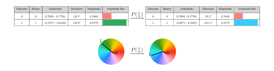
The effect of the \(P(\phi)\) gate on a pair of amplitudes.

The effect of the \(P(\phi)\) gate on a pair of probabilities with direction.

The effect of the \(P(\pi/3)\) gate on our example state.

The effect of the H-gate on a pair of amplitudes.

The effect of the H-gate on our example pair of amplitudes.

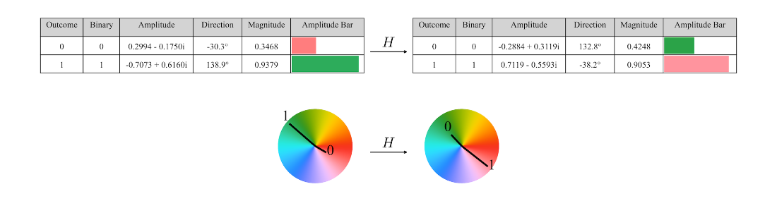
The effect of the H-gate on the default single-qubit state.

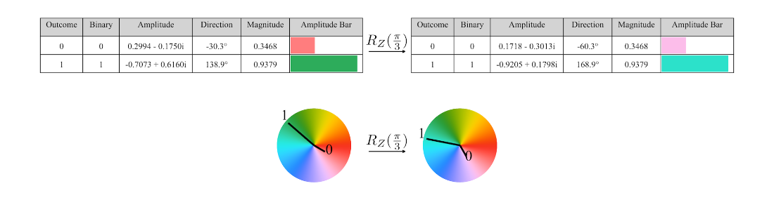
The effect of the \(R_Z\)-gate on a pair of amplitudes

The effect of the \(R_Z\)-gate on a pair of probabilities with direction

The effect of the \(R_Z(\frac{\pi}{3})\)-gate on our example pair of amplitudes.

The effect of the \(Y\)-gate on a pair of amplitudes

The effect of the Y-gate on a pair of probabilities with direction

The effect of the Y-gate on our example pair of amplitudes.

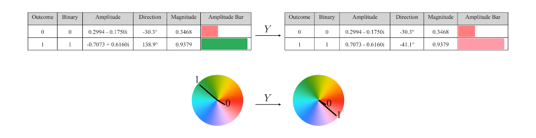
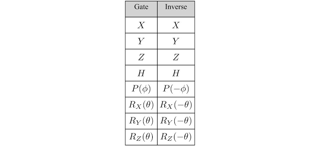
Table 3.9 Two-by-two matrix representations for the X, Y, Z, H, P, \(R_Z\) gates.

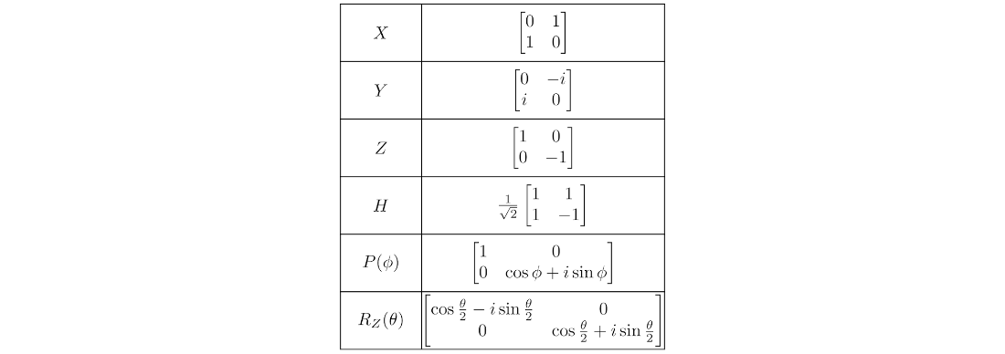
The effect of the \(R_X(\frac{\pi}{3})\)-gate on our example pair of amplitudes.

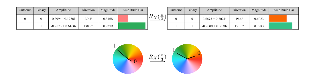
The effect of the \(R_Y(\frac{\pi}{3})\)-gate on our example pair of amplitudes.

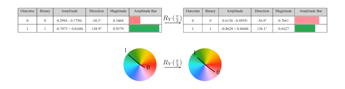
Table 3.10 Gate inverses.

The steps of a single-qubit quantum computation.

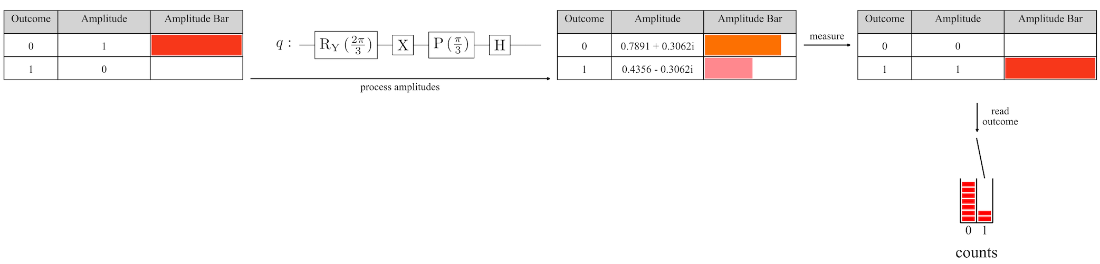
A circuit diagram representation of the gate sequence \(HP(\frac{\pi}{3})XR_Y(\frac{2\pi}{3})\).

Table 3.11 The table state of a single-qubit state after the transformations in figure 3.26.

Example single-qubit circuit.

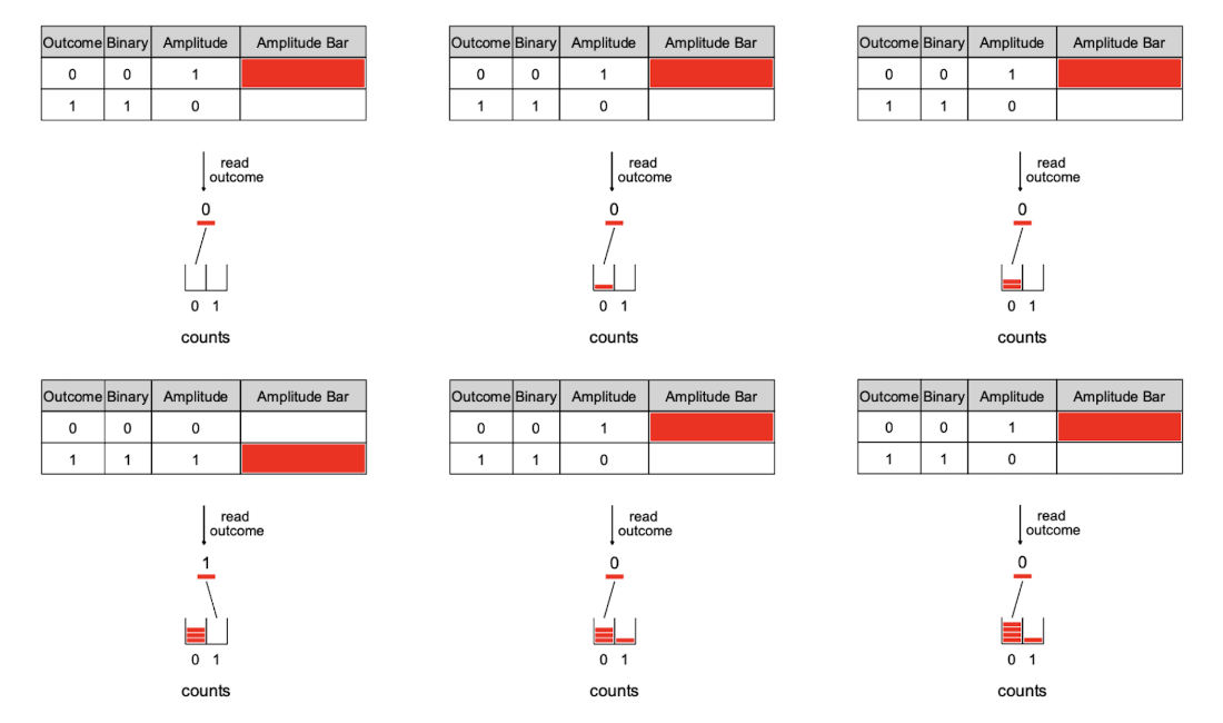
Mental model of the single-qubit circuit in figure 3.27, with counts of the outcomes from previous executions of the computation.

Ten measurements and the resulting outcome counts.

The Bernoulli distribution for \(p = 0.8\).

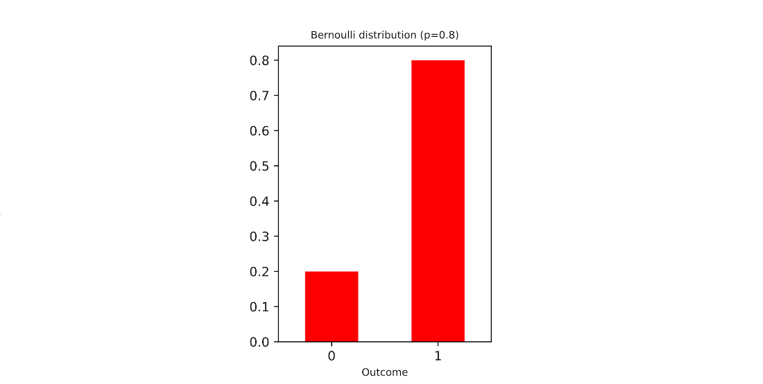
Table 3.12 The state table after encoding the value \(x = 273.5\) in a single-qubit state in the magnitude of outcome 0.

Table 3.13 The state table after encoding the value \(x = 273.5\) in a single-qubit state in the phase of the amplitude corresponding to outcome 1.

• Single-qubit computations are the simplest form of quantum computing. They are comparable to tossing a coin and have two possible outcomes.
• We can simulate a one-qubit computation using a two-element list of complex numbers. This list is initialized at the start, then undergoes simple transformations (known as single-qubit gates).
• The most common single-qubit gates are X, Y, Z, P, H, and rotations (denoted as \(R_X\), \(R_Y\), and \(R_Z\)). These rotations require an angle parameter.
• We can visualize the state of a single-qubit system with state tables that include amplitudes and other useful derived properties (directions, magnitudes, probabilities).
• Sequences of gates are called quantum circuits.
• Quantum computations are non-deterministic. When repeated, they yield different outcomes with distributions that reflect the state of the quantum system.
• The outcomes of a repeated quantum computation are aggregated into counts, which compose the typical output of a quantum computer.
• Single-qubit computations can be used to generate truly random numbers from Bernoulli distributions.

FAQ

from math import sqrt
def init_state():
    return [1, 0]

def prepare_state(*a):
    state = list(a)
    assert len(state) == 2
    assert abs(sum(abs(x)**2 for x in state) - 1) < 1e-9
    return state

from math import atan2, pi
z = 0.3 + 0.4j
mag = abs(z)              # 0.5
theta = atan2(z.imag, z.real)  # radians
deg = theta * 180 / pi

from math import cos, sin
def cis(theta): return cos(theta) + 1j*sin(theta)

z_new = cis(phi) * z_old  # rotate z_old by phi

def transform(state, gate):
    z0, z1 = state
    state[0] = gate[0][0]*z0 + gate[0][1]*z1
    state[1] = gate[1][0]*z0 + gate[1][1]*z1

from random import choices
from collections import Counter
probs = [abs(z)**2 for z in state]
samples = choices([0,1], probs, k=1000)
counts = Counter(samples)  # e.g., {0: 726, 1: 274}