4 Implementing a GPT model from Scratch To Generate Text

This chapter walks from a top-down sketch to a working, GPT-like language model that generates text token by token. Building on the prior chapter’s masked multi-head attention, it sets a clear target—recreating the “GPT‑2 small” configuration—and outlines how tokenization, token and positional embeddings, stacked transformer blocks, and a final projection layer fit together. The author adopts a pragmatic approach: start with a placeholder backbone to map inputs to logits, then progressively replace stubs with real components, aiming at an implementation that mirrors GPT‑2’s design while remaining easy to scale to larger variants.

The core building blocks are implemented and motivated in turn. Layer normalization is introduced to stabilize training (used in a pre-layer norm setup), followed by a feed-forward subnetwork that expands the embedding dimension by 4x, applies a GELU nonlinearity, and projects back to the model width. Residual (shortcut) connections are emphasized as crucial for healthy gradient flow in deep stacks. These pieces are composed into a reusable TransformerBlock that combines attention, dropout, layer norm, residual paths, and the GELU-based feed-forward. The full GPTModel then stacks multiple blocks between embeddings and an output head. The chapter also explains parameter accounting, the notion of weight tying in GPT‑2 (why “124M” counts differ from naive totals), and the resulting memory footprint, highlighting how large even a “small” LLM can be.

Finally, the chapter shows how model outputs (logits shaped by batch, sequence length, and vocabulary size) are turned into text with a simple greedy decoding loop that repeatedly selects the most probable next token and appends it to the context. This illustrates the end-to-end path from input text to generated output and clarifies why an untrained model produces gibberish—training is covered next. Throughout, the configuration remains the single source of truth (vocab size, context length, embedding width, heads, layers, dropout, and QKV bias), making it straightforward to scale the same codebase from GPT‑2 small to larger variants and to experiment with architectural options.

A mental model of the three main stages of coding an LLM, pretraining the LLM on a general text dataset, and finetuning it on a labeled dataset. This chapter focuses on implementing the LLM architecture, which we will train in the next chapter.

A mental model of a GPT model. Next to the embedding layers, it consists of one or more transformer blocks containing the masked multi-head attention module we implemented in the previous chapter.

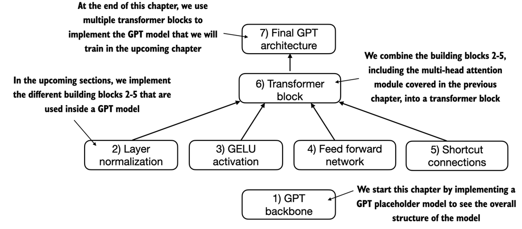
A mental model outlining the order in which we code the GPT architecture. In this chapter, we will start with the GPT backbone, a placeholder architecture, before we get to the individual core pieces and eventually assemble them in a transformer block for the final GPT architecture.

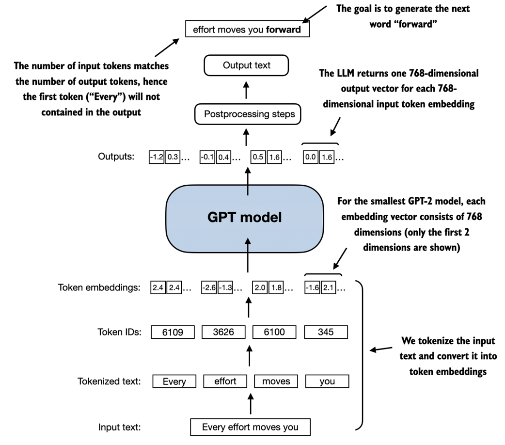
A big-picture overview showing how the input data is tokenized, embedded, and fed to the GPT model. Note that in our DummyGPTClass coded earlier, the token embedding is handled inside the GPT model. In LLMs, the embedded input token dimension typically matches the output dimension. The output embeddings here represent the context vectors we discussed in chapter 3.

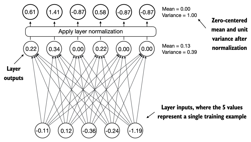
An illustration of layer normalization where the 5 layer outputs, also called activations, are normalized such that they have a zero mean and variance of 1.

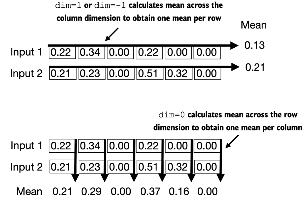
An illustration of the dim parameter when calculating the mean of a tensor. For instance, if we have a 2D tensor (matrix) with dimensions [rows, columns], using dim=0 will perform the operation across rows (vertically, as shown at the bottom), resulting in an output that aggregates the data for each column. Using dim=1 or dim=-1 will perform the operation across columns (horizontally, as shown at the top), resulting in an output aggregating the data for each row.

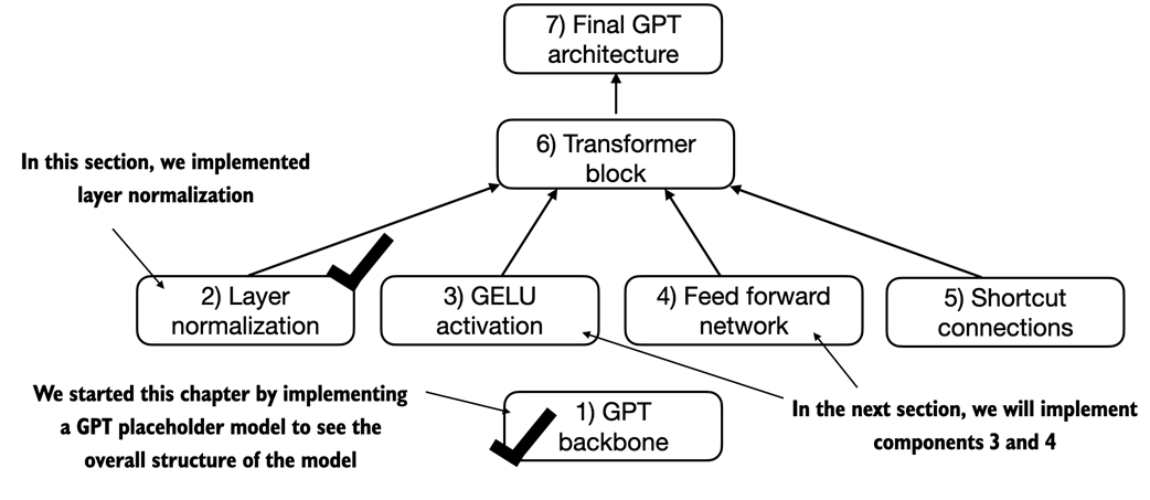
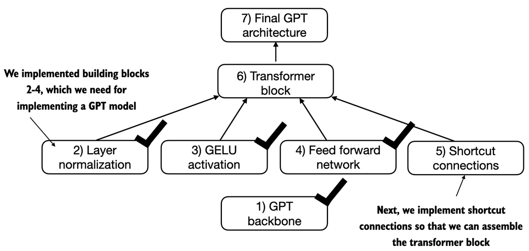
A mental model listing the different building blocks we implement in this chapter to assemble the GPT architecture.

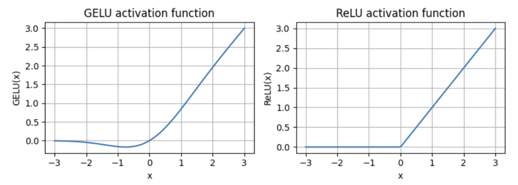
The output of the GELU and ReLU plots using matplotlib. The x-axis shows the function inputs and the y-axis shows the function outputs.

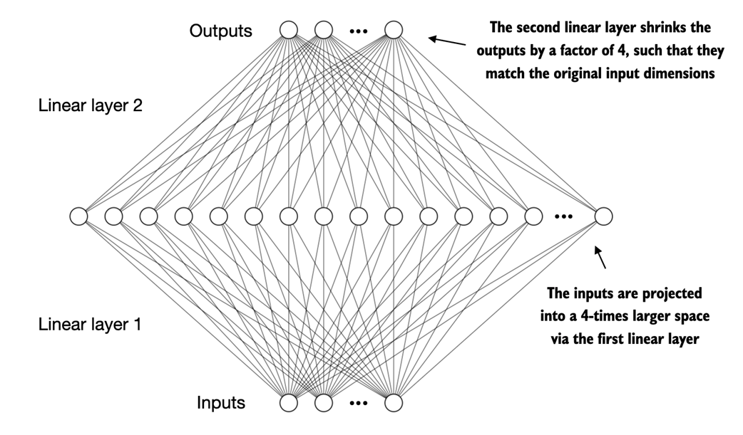
provides a visual overview of the connections between the layers of the feed forward neural network. It is important to note that this neural network can accommodate variable batch sizes and numbers of tokens in the input. However, the embedding size for each token is determined and fixed when initializing the weights.

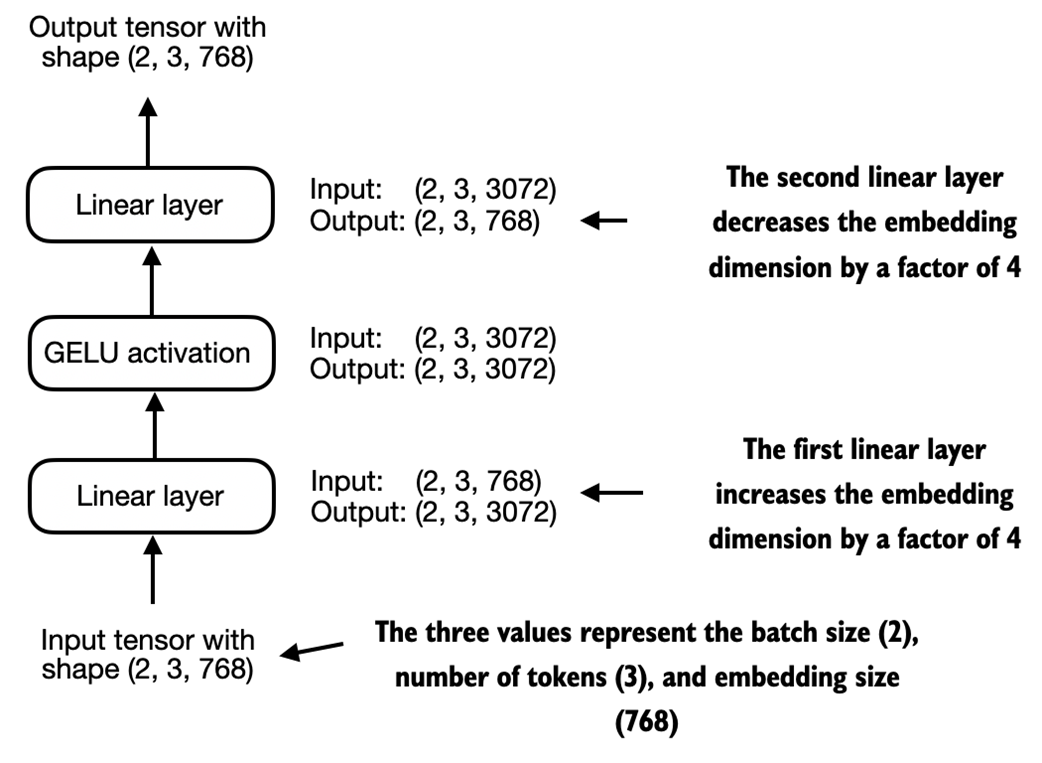
An illustration of the expansion and contraction of the layer outputs in the feed forward neural network. First, the inputs expand by a factor of 4 from 768 to 3072 values. Then, the second layer compresses the 3072 values back into a 768-dimensional representation.

A mental model showing the topics we cover in this chapter, with the black checkmarks indicating those that we have already covered.

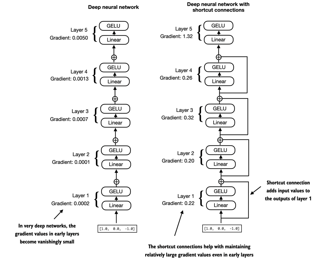
A comparison between a deep neural network consisting of 5 layers without (on the left) and with shortcut connections (on the right). Shortcut connections involve adding the inputs of a layer to its outputs, effectively creating an alternate path that bypasses certain layers. The gradient illustrated in Figure 1.1 denotes the mean absolute gradient at each layer, which we will compute in the code example that follows.

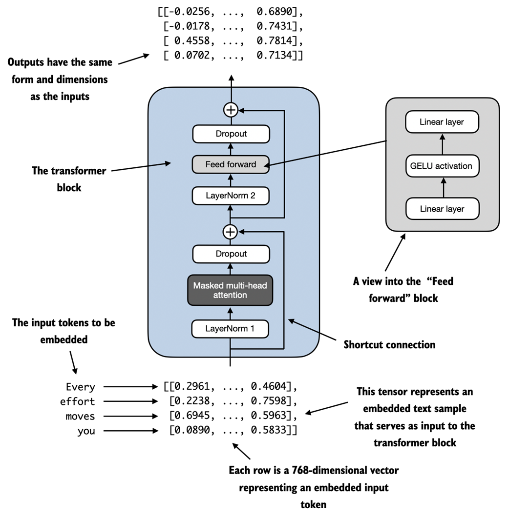
An illustration of a transformer block. The bottom of the diagram shows input tokens that have been embedded into 768-dimensional vectors. Each row corresponds to one token's vector representation. The outputs of the transformer block are vectors of the same dimension as the input, which can then be fed into subsequent layers in an LLM.

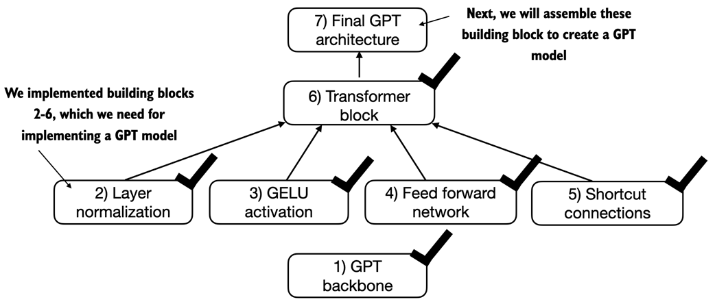
A mental model of the different concepts we have implemented in this chapter so far.

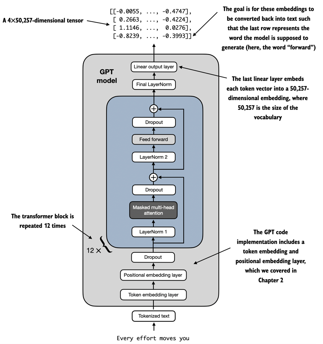
An overview of the GPT model architecture. This figure illustrates the flow of data through the GPT model. Starting from the bottom, tokenized text is first converted into token embeddings, which are then augmented with positional embeddings. This combined information forms a tensor that is passed through a series of transformer blocks shown in the center (each containing multi-head attention and feed forward neural network layers with dropout and layer normalization), which are stacked on top of each other and repeated 12 times.

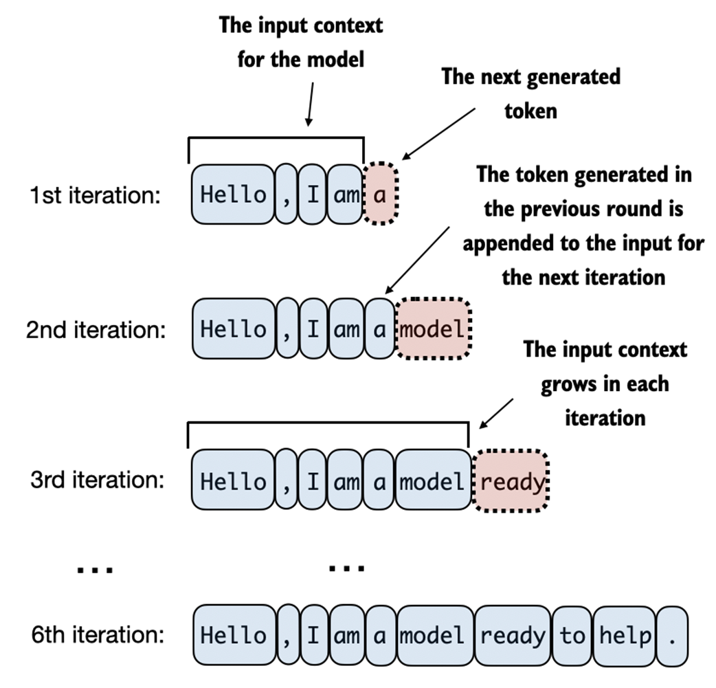
This diagram illustrates the step-by-step process by which an LLM generates text, one token at a time. Starting with an initial input context ("Hello, I am"), the model predicts a subsequent token during each iteration, appending it to the input context for the next round of prediction. As shown, the first iteration adds "a", the second "model", and the third "ready", progressively building the sentence.

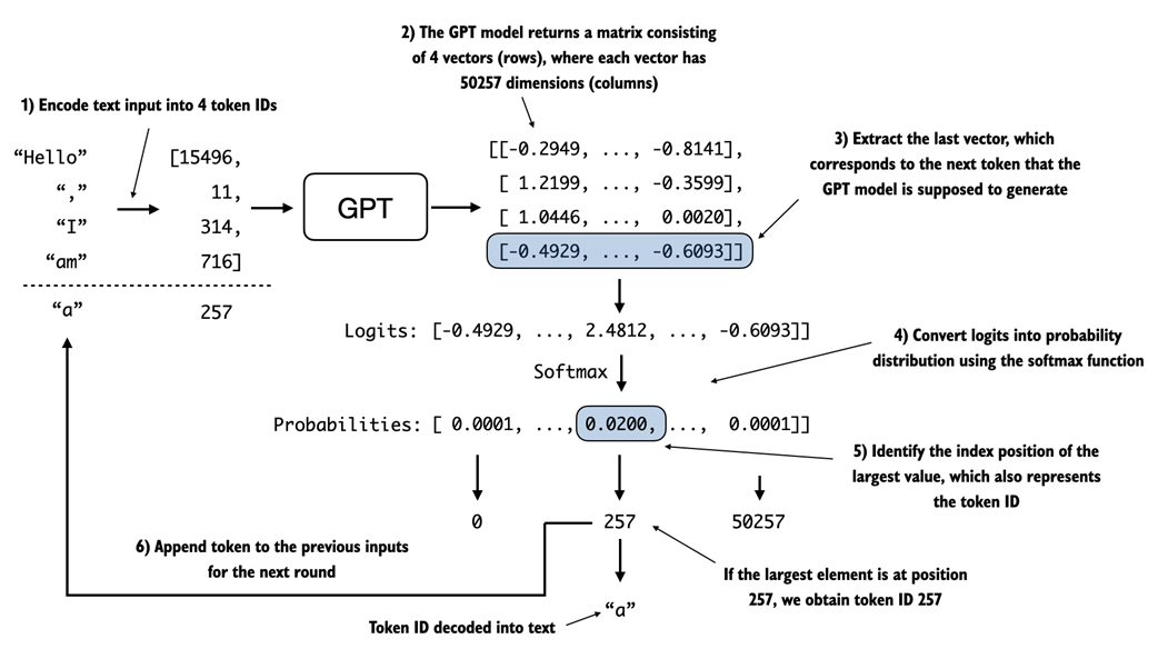
details the mechanics of text generation in a GPT model by showing a single iteration in the token generation process. The process begins by encoding the input text into token IDs, which are then fed into the GPT model. The outputs of the model are then converted back into text and appended to the original input text.

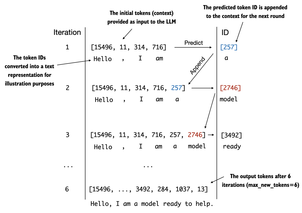
An illustration showing six iterations of a token prediction cycle, where the model takes a sequence of initial token IDs as input, predicts the next token, and appends this token to the input sequence for the next iteration. (The token IDs are also translated into their corresponding text for better understanding.)

• Layer normalization stabilizes training by ensuring that each layer's outputs have a consistent mean and variance.
• Shortcut connections are connections that skip one or more layers by feeding the output of one layer directly to a deeper layer, which helps mitigate the vanishing gradient problem when training deep neural networks, such as LLMs.
• Transformer blocks are a core structural component of GPT models, combining masked multi-head attention modules with fully connected feed-forward networks that use the GELU activation function.
• GPT models are LLMs with many repeated transformer blocks that have millions to billions of parameters.
• GPT models come in various sizes, for example, 124, 345, 762, and 1542 million parameters, which we can implement with the same GPTModel Python class.
• The text generation capability of a GPT-like LLM involves decoding output tensors into human-readable text by sequentially predicting one token at a time based on a given input context.
• Without training, a GPT model generates incoherent text, which underscores the importance of model training for coherent text generation, which is the topic of subsequent chapters.

FAQ