Appendix A. Introduction to PyTorch

This appendix is a practical primer that equips readers to put deep learning into practice with PyTorch as the core tool for building large language models from scratch. It introduces PyTorch’s goals and strengths—combining usability with flexibility—and focuses on the essential features needed throughout the book rather than exhaustive coverage. Readers are guided through environment setup and installation choices, including CPU/GPU variants and version compatibility, with the aim of establishing a reliable, reproducible workspace before moving on to model implementation and training.

The chapter centers on PyTorch’s three pillars: tensors, automatic differentiation, and deep learning utilities. It explains tensors as the fundamental data container (covering ranks, dtypes, shapes, reshaping, transposition, and matrix multiplication) and shows how PyTorch mirrors NumPy while adding GPU support. It then introduces computation graphs and autograd to compute gradients automatically via backward passes, enabling backpropagation without manual calculus. Building on this, the text demonstrates how to define neural networks by subclassing torch.nn.Module, structuring layers (often with Sequential), running forward passes to produce logits, selecting suitable losses and optimizers, and executing the canonical training loop (zero_grad → backward → step) with proper train/eval modes, no_grad for inference, and model persistence via state_dict save/load.

Efficient data handling is addressed through custom Dataset classes and DataLoader configuration, including batching, shuffling, drop_last, and num_workers trade-offs to avoid CPU bottlenecks. The chapter concludes with performance optimization: moving tensors and models across devices, running on a single GPU with minimal code changes, and scaling to multiple GPUs using DistributedDataParallel with DistributedSampler and synchronized gradients. Along the way, it stresses practical considerations—accuracy evaluation, logits-to-probabilities conversion when needed, and careful resource management—so readers are prepared to train, evaluate, save, and scale PyTorch models effectively.

Figure A.1 PyTorch's three main components include a tensor library as a fundamental building block for computing, automatic differentiation for model optimization, and deep learning utility functions, making it easier to implement and train deep neural network models.

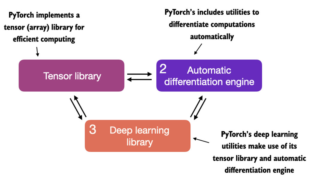
Figure A.2 Deep learning is a subcategory of machine learning that is focused on the implementation of deep neural networks. In turn, machine learning is a subcategory of AI that is concerned with algorithms that learn from data. AI is the broader concept of machines being able to perform tasks that typically require human intelligence.

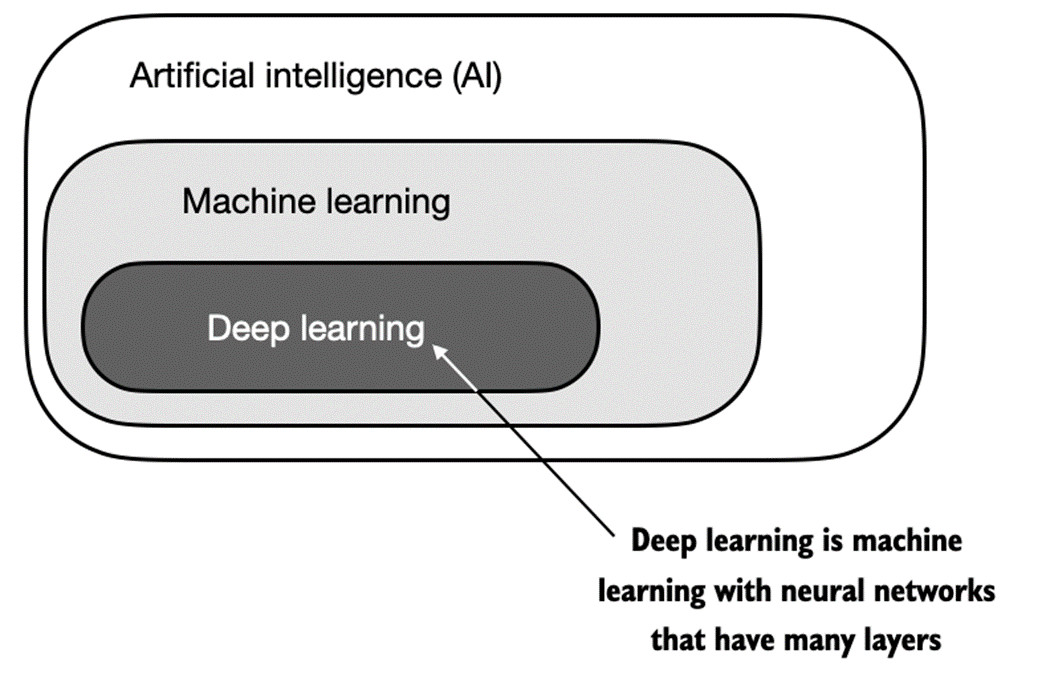
Figure A.3 The supervised learning workflow for predictive modeling consists of a training stage where a model is trained on labeled examples in a training dataset. The trained model can then be used to predict the labels of new observations.

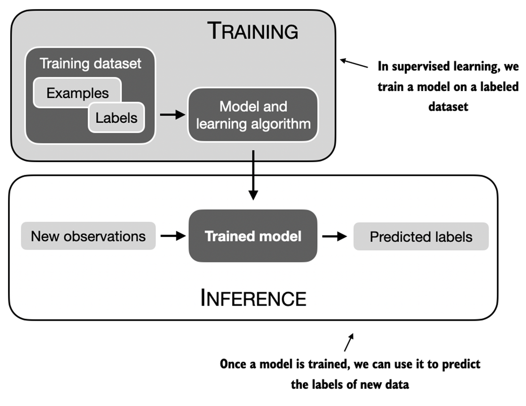
Figure A.4 Access the PyTorch installation recommendation on https://pytorch.org to customize and select the installation command for your system.

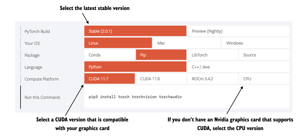
Figure A.5 Select a GPU device for Google Colab under the Runtime/Change runtime type menu.

Figure A.6 An illustration of tensors with different ranks. Here 0D corresponds to rank 0, 1D to rank 1, and 2D to rank 2. Note that a 3D vector, which consists of 3 elements, is still a rank 1 tensor.

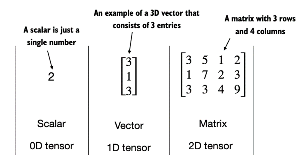
Figure A.7 A logistic regression forward pass as a computation graph. The input feature x1 is multiplied by a model weight w1 and passed through an activation function σ after adding the bias. The loss is computed by comparing the model output a with a given label y.

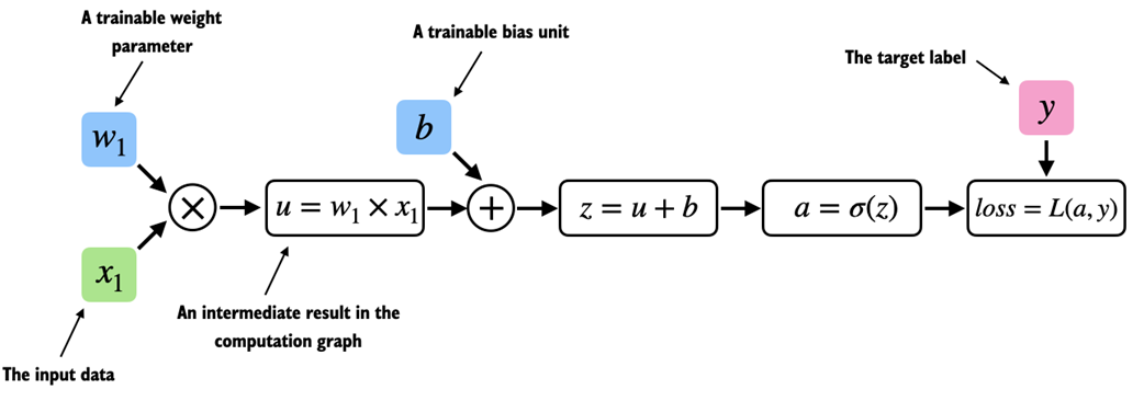
Figure A.8 The most common way of computing the loss gradients in a computation graph involves applying the chain rule from right to left, which is also called reverse-model automatic differentiation or backpropagation. It means we start from the output layer (or the loss itself) and work backward through the network to the input layer. This is done to compute the gradient of the loss with respect to each parameter (weights and biases) in the network, which informs how we update these parameters during training.

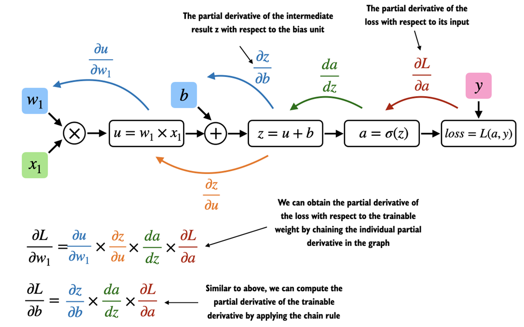
Figure A.9 An illustration of a multilayer perceptron with 2 hidden layers. Each node represents a unit in the respective layer. Each layer has only a very small number of nodes for illustration purposes.

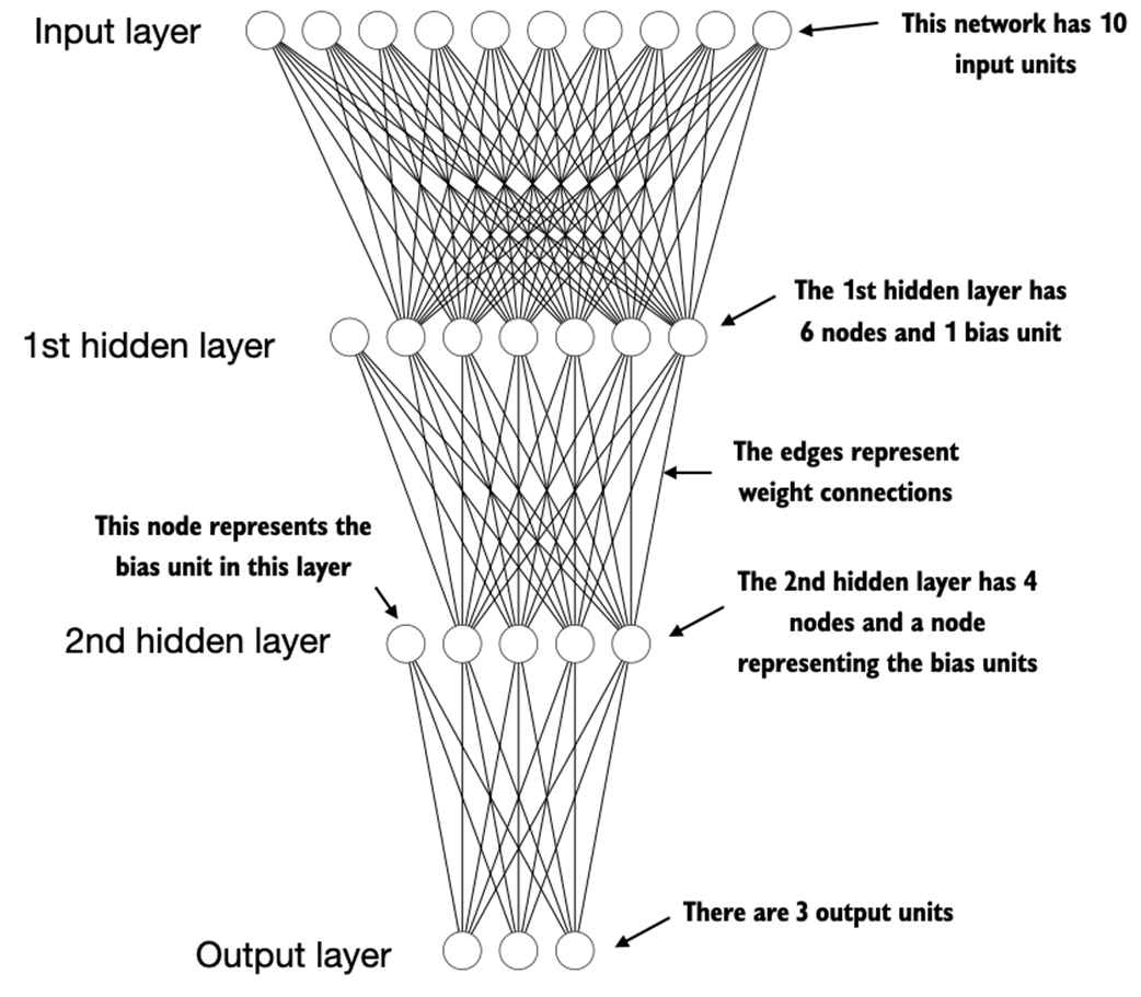
Figure A.10 PyTorch implements a Dataset and a DataLoader class. The Dataset class is used to instantiate objects that define how each data record is loaded. The DataLoader handles how the data is shuffled and assembled into batches.

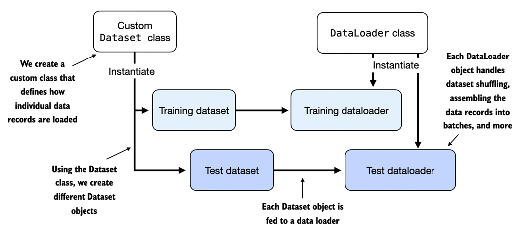
Figure A.11 Loading data without multiple workers (setting num_workers=0) will create a data loading bottleneck where the model sits idle until the next batch is loaded as illustrated in the left subpanel. If multiple workers are enabled, the data loader can already queue up the next batch in the background as shown in the right subpanel.

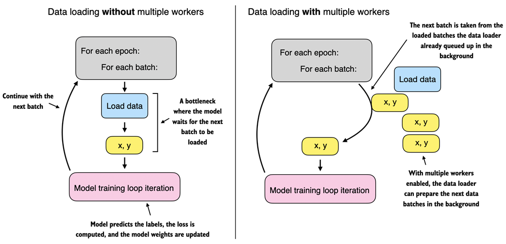
Figure A.12 The model and data transfer in DDP involves two key steps. First, we create a copy of the model on each of the GPUs. Then we divide the input data into unique minibatches that we pass on to each model copy.

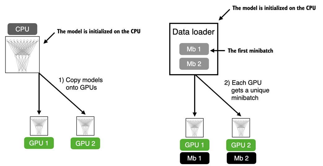
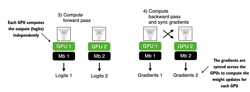
Figure A.13 The forward and backward pass in DDP are executed independently on each GPU with its corresponding data subset. Once the forward and backward passes are completed, gradients from each model replica (on each GPU) are synchronized across all GPUs. This ensures that every model replica has the same updated weights.

FAQ

import torch
print(torch.__version__)

import torch
print(torch.cuda.is_available())  # True means CUDA GPU usable

import torch
print(torch.backends.mps.is_available())  # True means MPS usable

import torch
t0 = torch.tensor(1)              # 0D
t1 = torch.tensor([1, 2, 3])      # 1D
t2 = torch.tensor([[1, 2], [3, 4]])  # 2D

t = torch.tensor([1, 2, 3])       # int64
t = t.to(torch.float32)           # float32

x = torch.tensor([[1, 2, 3], [4, 5, 6]])
print(x.shape)      # torch.Size([2, 3])
print(x.T)          # transpose
print(x @ x.T)      # 2x3 @ 3x2 -> 2x2

import torch, torch.nn.functional as F
x = torch.tensor([1.1])
w = torch.tensor([2.2], requires_grad=True)
b = torch.tensor([0.0], requires_grad=True)
y = torch.tensor([1.0])

a = torch.sigmoid(x * w + b)
loss = F.binary_cross_entropy(a, y)
loss.backward()
print(w.grad, b.grad)  # gradients

class NeuralNetwork(torch.nn.Module):
    def __init__(self, num_inputs, num_outputs):
        super().__init__()
        self.layers = torch.nn.Sequential(
            torch.nn.Linear(num_inputs, 30), torch.nn.ReLU(),
            torch.nn.Linear(30, 20),         torch.nn.ReLU(),
            torch.nn.Linear(20, num_outputs)
        )
    def forward(self, x):
        return self.layers(x)  # logits

with torch.no_grad():
    probs = torch.softmax(model(x), dim=1)

from torch.utils.data import DataLoader
loader = DataLoader(dataset=train_ds,
                    batch_size=32,
                    shuffle=True,
                    drop_last=True,   # avoid tiny last batch
                    num_workers=4)    # parallel data loading

# save
torch.save(model.state_dict(), "model.pth")
# load
model = NeuralNetwork(in_dim, out_dim)
model.load_state_dict(torch.load("model.pth"))

device = torch.device("cuda" if torch.cuda.is_available() else "cpu")
model = model.to(device)
for features, labels in train_loader:
    features, labels = features.to(device), labels.to(device)