Overview

7 Sampling from Data Streams

This chapter motivates sampling as a core task for fast, approximate analytics over massive data streams. It frames streaming models—landmark streams and sliding windows—and explains the goal: maintain small, continually updated samples that enable near-real-time answers with controllable error and small failure probability, all in one pass and with sublinear memory. Building on ideas from database sampling and online aggregation, the text anchors each method in an IP-address fingerprinting use case, emphasizing practical constraints like de-duplication, single-pass processing, and low-latency querying.

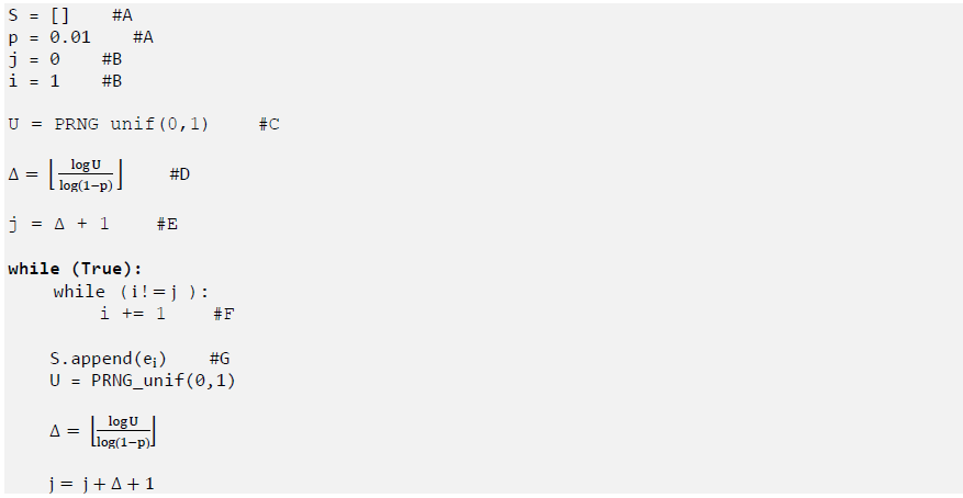
For landmark streams, the chapter first covers Bernoulli sampling (and Poisson as a generalized, weighted variant). It highlights a skip-based implementation that reduces calls to pseudo-random generators and notes advantages such as natural parallelizability across substreams, while stressing the drawback of an unbounded, random sample size. Reservoir sampling solves that by keeping a fixed-size simple random sample: early elements fill the reservoir, later ones probabilistically replace existing items. An efficient implementation uses inverse transform sampling, acceptance–rejection, and “squeezing” to jump over non-included elements. The chapter then introduces biased reservoir sampling to favor recency, modeling “residing probability” with an exponential, memoryless decay controlled by a parameter that tunes the speed of aging. It provides bounds on expected sample size, a simple maintenance rule that mixes replacement with appends based on reservoir occupancy, and a throttled variant for tighter memory budgets.

For sliding windows, two specialized methods maintain freshness as items age out. Chain Sampling targets sequence-based windows by running k independent chains: each chain maintains a current item and a preselected successor to inherit the sample exactly when the current one expires, yielding at each moment a sample of size k with replacement using small, bounded memory. Priority Sampling addresses timestamp-based windows by assigning each arrival a random priority; the current sample is the highest-priority item within the window, while a priority-ordered successor list ensures immediate, correct handover at expiration with modest expected memory. A comparative study using an R stream framework shows that biased reservoir sampling adapts quickly to sudden distribution shifts, while standard reservoir sampling lags due to its uniform weighting of old and new data. The chapter closes with guidance on choosing the aging rate to match an application’s effective horizon and notes practical support in R and Python for prototyping and testing streaming samplers.

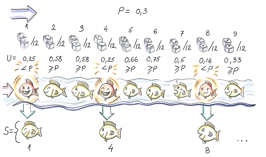
You can see how first, fourth and eight element of the stream are included in the sample, since the corresponding pseudo-random value uniform on [0,1] turned out less than p=0.3.
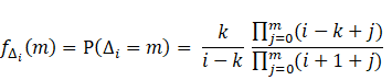
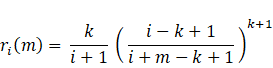
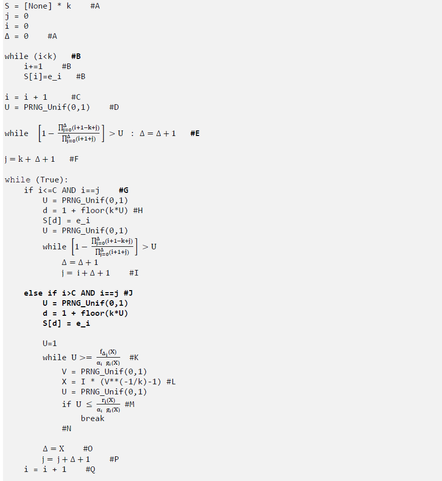
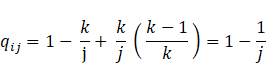
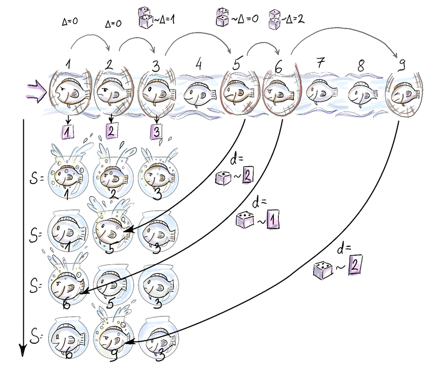
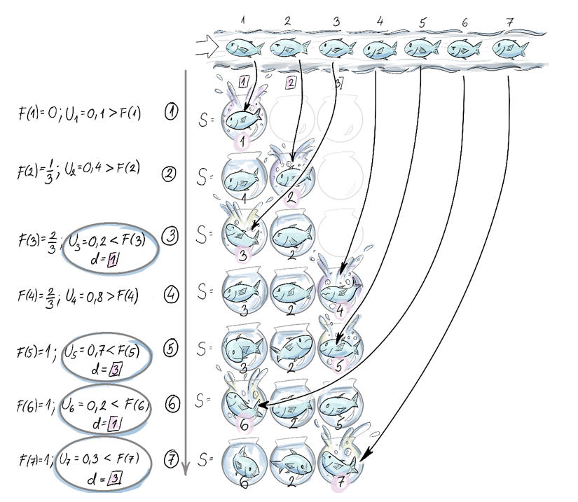
: The figure shows the content of the reservoir after each of the first seven arrivals. First three elements are included in the sample deterministically. Subsequently, is skipped (this corresponds to the number of elements to skip, after is included being 1). is then randomly replaces in the reservoir . Next element, is included at the random position 1 in the reservoir, and replaces (notice that this means that was 0). is definitely bigger than 0, since at least one element, , is skipped.
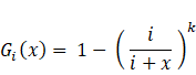
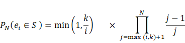
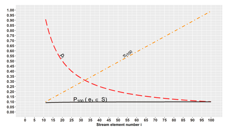
: We can see the balance between probabilities of inclusion (red, longdash line,) and probabilities of “removal up to the time point N=100” (orange, dotdash line) reflected in (black line) being approximately constant for all elements seen so far (when the reservoir is of size 10). This means that each element, no matter when it has been seen, has the same chance of being in the sample.
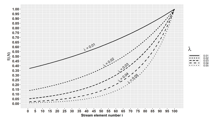
: Notice that for we need 100 elements to reduce f(i,N) by the factor of 0.36, while for this number is 50. So the higher the , easier it is to forget old elements.
: The figure shows the content of the reservoir for first 7 arrivals under the the biased reservoir sampling strategy.
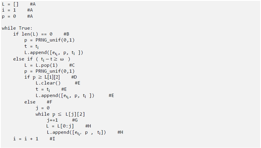
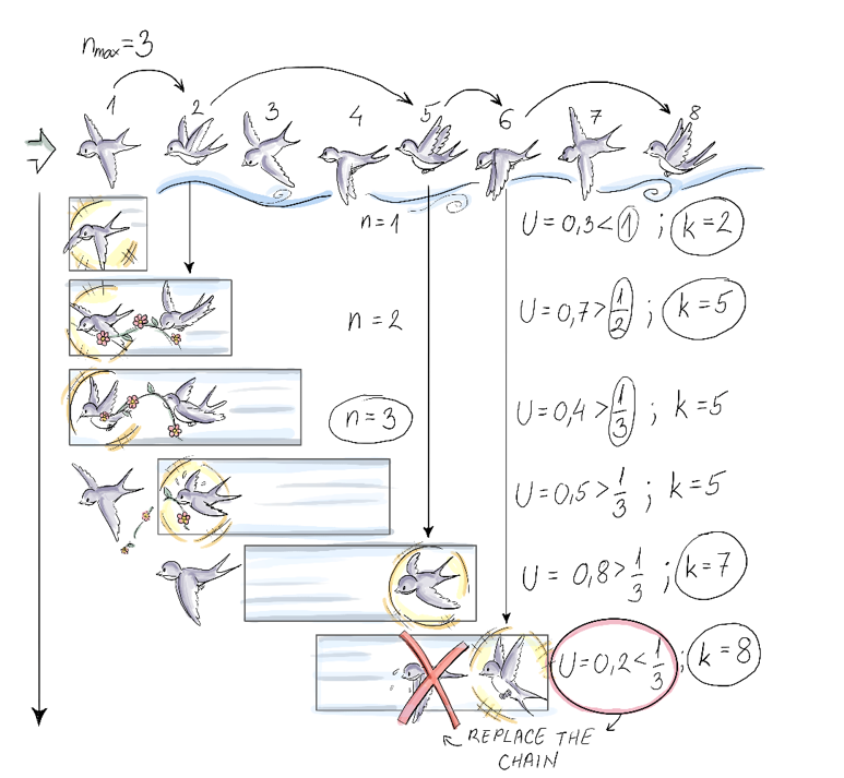
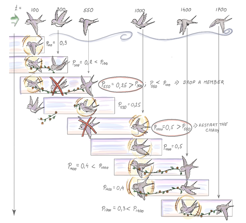
: Figure shows the content of the chain (list L) for the first 7 elements from a sequence-based windowed stream of size n=3.
: Figure shows content of the list of successors and the current sample for first 6 arrival times in ms for a timestamp-based window of length 600 ms.
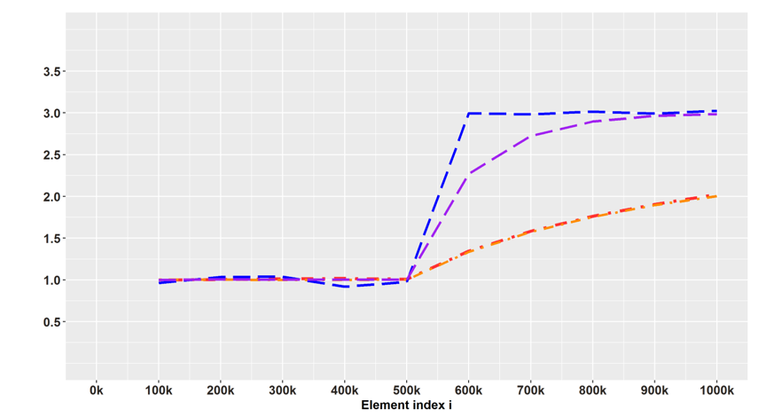
Dashed lines (purple and blue) connect sample averages of samples selected using biased reservor sampling. Blue (upper) with and for the purple (lower) dashed line. Dot-dashed lines (red and range) track sample averages at every 100k new elements for two unbiased reservoir sample sizes.
 Summary

  • We have gotten to know five algorithms for sampling from a data stream (three for landmark streams and two for windowed streams). Bernoulli sampling is a very simple and representative sampling algorithm, but if you want to use it, you have to think about some sample size curbing strategy, without introducing much bias.
  • Reservoir sampling solved our problem of variable sample size and delivered a SRS from elements seen so far at any moment. If we would want to accentuate more recent elements in our sample, biased reservoir sampling would be one way to go. Here, we need to think about our desired speed of aging factor and how it relates to our available space. This depends on the realistic parameters that you face in your own application.
  • The other option to accentuate recently arrived elements in the stream is via sliding window. If we decide that we need to sample from that window due to its size, we learned how to implement chain sampling for sequence-based windows and priority sampling for time-based windows.
  • We saw how biased reservoir sampling in our simulation managed to adjust to sudden shift in concept, while reservoir sampling was unable to react to this change, and led to biased answer of the query about the current / recent true average of the stream data. You do need to adjust the speed of aging parameter though, so that it suits notion of sufficient recency for your particular use-case.

FAQ

What is a landmark stream and why is sampling from it simpler than from a windowed stream?In a landmark stream, items arrive continuously and never “age out” of consideration; you aim to keep a representative sample of everything seen so far. Because nothing leaves the population, you only worry about adding elements, not removing them. That makes single-pass, small-memory samplers (like Bernoulli and reservoir sampling) easier than windowed settings, where elements must be removed as the window slides.
How does Bernoulli sampling work on a data stream, and how can we make it efficient?Bernoulli sampling flips a biased coin for each incoming item and includes it with a fixed probability p, yielding a representative but random-size sample. To reduce pseudo-random number generator (PRNG) calls, you can generate geometric “skips”: compute how many items to skip before the next inclusion using inverse-transform sampling, and only draw randomness when you actually include an item. This preserves correctness while lowering per-element overhead and latency.
When should I prefer Poisson (weighted) sampling over plain Bernoulli sampling?Use Poisson sampling when items should have different inclusion probabilities (for example, proportional to estimated frequency or value magnitude). This enables unbiased estimators like Horvitz–Thompson and can reduce variance by oversampling influential items. The trade-off is higher implementation complexity (e.g., generating nontrivial skips) and, like Bernoulli, a sample size that fluctuates over time.
What’s the main drawback of Bernoulli/Poisson sampling, and why might that matter in production?The sample size is a random variable and can grow without bound on a long-lived landmark stream. Ad hoc “curtailing” (e.g., truncating the sample or switching algorithms past a threshold) typically introduces bias that’s hard to correct analytically. If you need predictable space usage without post hoc bias, use reservoir sampling.
How does Reservoir Sampling maintain a uniform sample of fixed size k from a stream?Reservoir sampling fills a buffer with the first k items, then for the ith item (i > k) includes it with probability k/i by replacing a random element in the reservoir. This yields a simple random sample (without replacement) of size k from all items seen so far. Efficient implementations also generate “skips” between replacements to minimize per-item work; time is linear in items processed and space is O(k). Bernoulli sampling, in contrast, is trivially parallelizable across shards (same p per shard, then union), while reservoir sampling requires careful merging or centralized coordination.
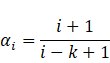
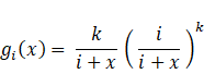
What is Biased Reservoir Sampling and how do I choose the recency parameter?Biased reservoir sampling tilts inclusion toward recent items by making an element’s “probability of still residing in the reservoir” decay with its age, often via an exponential decay controlled by a rate λ. Larger λ “forgets” faster (more responsiveness, less history), while smaller λ retains more history (slower adaptation). Practical tuning links λ to the effective horizon you care about (for instance, the number of arrivals over a day) and to memory limits; expected sample size grows roughly with 1/λ, so ensure the implied maximum fits your buffer. Some implementations use a COP (occupied proportion) control to manage whether new items append or replace an existing one.
What accuracy notion does the chapter use for approximate answers from samples?Approximate answers are evaluated by an error tolerance (absolute or relative) together with a small failure probability. Informally, the algorithm should return an answer within the target error most of the time, using a single pass and a sample whose size is polylogarithmic in the stream length (or in the window size for windowed streams). These criteria guide comparisons among streaming sampling methods under strict time/space constraints.
How do I sample uniformly from a sequence-based sliding window without storing the whole window?Chain sampling keeps a sample of size 1 along with a “chain” of designated successors that will take over when the current sample ages out. Running k independent chains in parallel yields a sample of size k from the current window; collectively this is a simple random sample with replacement. The chains remain short in expectation, so memory stays small while updates are constant-time on average per arrival and per expiration.
How do I maintain a uniform sample from a timestamp-based window where the item count is unknown?Priority sampling assigns each arriving item a random priority in (0,1) and treats the maximum-priority item within the current time window as the sample. A small, priority-ordered successor list is maintained so that when the current sample expires, the next-highest surviving priority takes over. For k samples, maintain k independent lists (one per sample); expected memory is small (proportional to k) with high-probability bounds on list growth. Ensure inter-arrival times don’t exceed the window length, or augment with periodic expiration checks.
Which tools can I use to try these algorithms quickly in practice?The R package “stream” provides data stream objects (DSD) and tasks (DST); function DSC_Sample implements both reservoir and biased reservoir sampling, with an update() call to ingest new batches. For biased reservoir sampling in that package, the aging rate parameter is tied to the chosen sample size (faster decay for smaller targets). In Python, you can prototype streaming via a lightweight Kafka demo that replays CSV time series, or build production-grade apps with Faust; both are useful for feeding a live stream into your sampler.

pro $24.99 per month

  • access to all Manning books, MEAPs, liveVideos, liveProjects, and audiobooks!
  • choose one free eBook per month to keep
  • exclusive 50% discount on all purchases
  • renews monthly, pause or cancel renewal anytime

lite $19.99 per month

  • access to all Manning books, including MEAPs!

team

5, 10 or 20 seats+ for your team - learn more


choose your plan

team

monthly
annual
$49.99
$499.99
only $41.67 per month
  • five seats for your team
  • access to all Manning books, MEAPs, liveVideos, liveProjects, and audiobooks!
  • choose another free product every time you renew
  • choose twelve free products per year
  • exclusive 50% discount on all purchases
  • renews monthly, pause or cancel renewal anytime
  • renews annually, pause or cancel renewal anytime
  • Algorithms and Data Structures for Massive Datasets ebook for free

choose your plan

team

monthly
annual
$49.99
$499.99
only $41.67 per month
  • five seats for your team
  • access to all Manning books, MEAPs, liveVideos, liveProjects, and audiobooks!
  • choose another free product every time you renew
  • choose twelve free products per year
  • exclusive 50% discount on all purchases
  • renews monthly, pause or cancel renewal anytime
  • renews annually, pause or cancel renewal anytime
  • Algorithms and Data Structures for Massive Datasets ebook for free