6 Streaming Data: Bringing Everything Together
This chapter zooms out from individual sketching algorithms to show how they live inside real-world streaming data systems. It contrasts the streaming model with traditional databases: data rushes past limited working memory, real-time insights are computed on-the-fly, and only archival storage holds full history that is too slow for interactive queries. Within this setting, approximate, probabilistic synopses enable continuous and ad‑hoc queries under tight time and space budgets. The chapter’s goal is to connect the algorithmic view to the practical pipeline where data is produced, queued, analyzed, and finally consumed.
Through meta-examples, the text maps algorithms onto the tiers of a streaming pipeline. Sampling requests in the analysis tier immediately exposes upstream needs like fast de-duplication in message queuing, naturally suggesting Bloom filter–based solutions. A Bloom-join shows how filters minimize cross-system data movement when joining clickstreams in a distributed file system with transactions in an enterprise warehouse. For infrastructure health, Count-Min Sketch detects heavy hitters for network traffic monitoring and broker load balancing, while HyperLogLog supports cardinality tasks. The result is a system-level perspective where Bloom filters, Count-Min Sketches, HyperLogLogs, and sampling interact across tiers to deliver timely, approximate answers.
The chapter then outlines the core constraints and concepts that shape streaming algorithms: one-pass processing, small time and small space, and the practical meaning of near real-time. It introduces concept shifts and drifts and motivates windowing—especially sliding windows—as a principled way to emphasize recency over stale data in infinite streams. Finally, it revisits sampling theory to prepare for stream sampling: distinguishing representative from biased sampling, analyzing selection probabilities, and using scale-up estimators of the Horvitz–Thompson type to infer totals and averages. These foundations tie algorithm design to pipeline realities and set the stage for the more technical developments to follow.
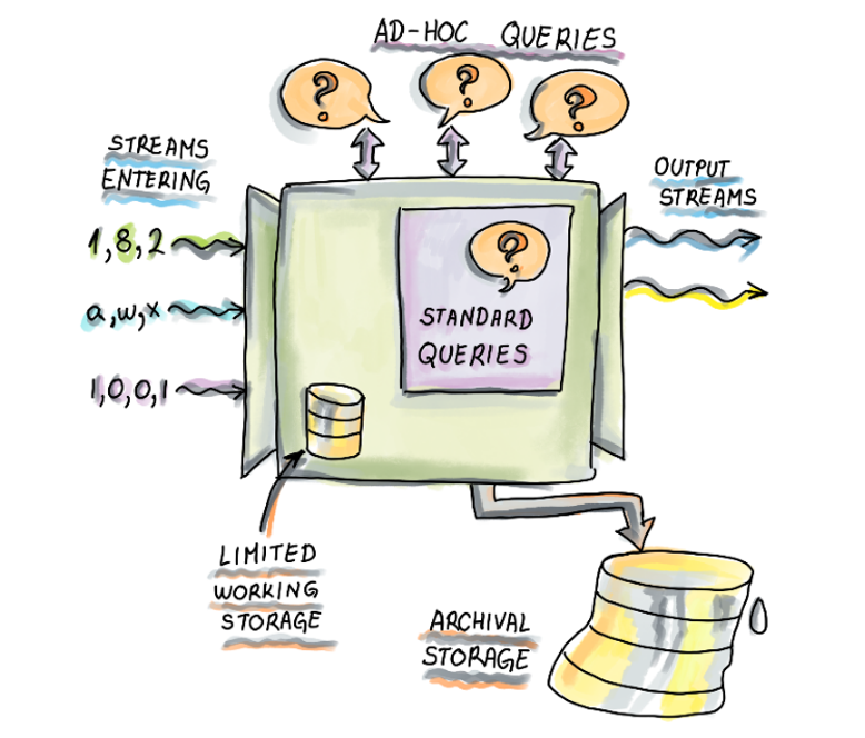
: Streaming data model. The streaming data model differs from the traditional database management system in that data passes through the processor and a small amount of working storage, and it is either never stored, or it is stored into the archival storage that is usually too large and slow to be indexed and searched. Items can be found there but we should not count on doing it often and quickly. All the real-time analysis is done on-the-fly. There are standard (or standing) queries, ones that need to be computed all the time, and ad-hoc queries, that show up at unexpected times and their content is externally controlled.
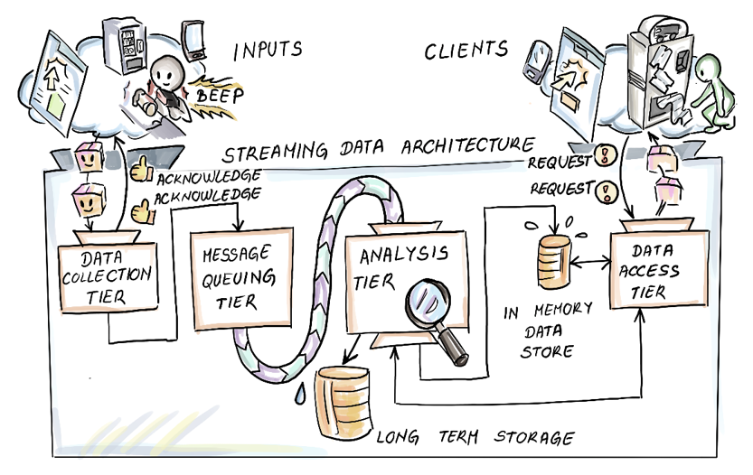
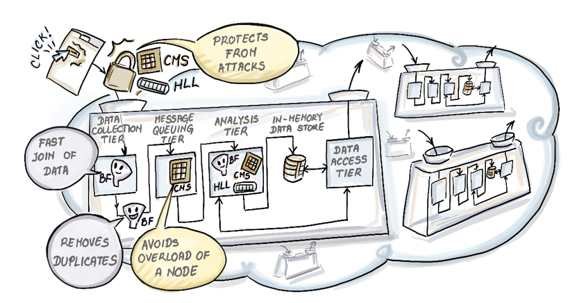
: The general model of a streaming data pipeline is shown. Data producers are initiating connections by interacting with retailer’s application.
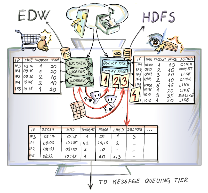
: Figure shows the pre-join communication between Enterprise Data Warehouse (EDW) implemented with fast parallel database (on the left) and a Hadoop Distributed File System (HDFS) (on the right). Before the data for financial transactions is sent from EDW side, exchange of Bloom Filters that both storage systems make for the mutual join key (IP address) is made. Bloom filters are used by each side as a criterion to identify tuples that will participate in the final-join. HDFS can then shuffle only necessary data among its nodes and move the minimum of data to the node that will execute the join to come. EDW will identify which IP addresses didn’t appear in HDFS and send only those that will participate in the final join. This way, purchase data is augmented with the click-stream component from that IP address and can further be used as a data source in a hybrid streaming data pipeline.
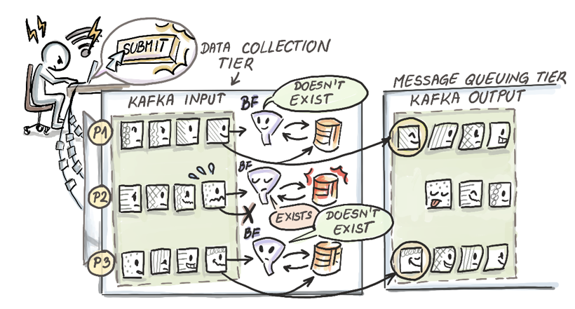
: Intermediate nodes connected to fast databases implementing de-duplication to remove the repeated messaging instances in a streaming data pipeline. Each node keeps a Bloom Filter of messages it saved and at arrival of the next message ID checks the message ID hash against its Bloom Filter. In case the Bloom Filter reports that the message already exists, this message with its data is discarded, otherwise the message is saved and propagated on to the message queuing tier.
: Figure shows a cloud computing architecture servicing different client data pipelines. Network traffic monitoring application installed to monitor communication of data producers (or any communication attempts originating outside of the cloud) is implemented with the help of a Count-Min Sketch. CMS identifies network flows that exhibit flow rates above a certain pre-determined threshold and acts accordingly. Similar problem of load balancing between the brokers of the message queuing tier is solved analogously by applying another CMS at the load balancer node in message queuing tier. Notice that both of these CMS are operating on the package / message headers and that the payload of the packets / messages, namely data on clicks issued by the user are not yet analyzed until they reach the analysis tier. There with the business problem at hand, other Bloom filters, Hyper-log-logs, sampling procedures or other synopsis are calculated.
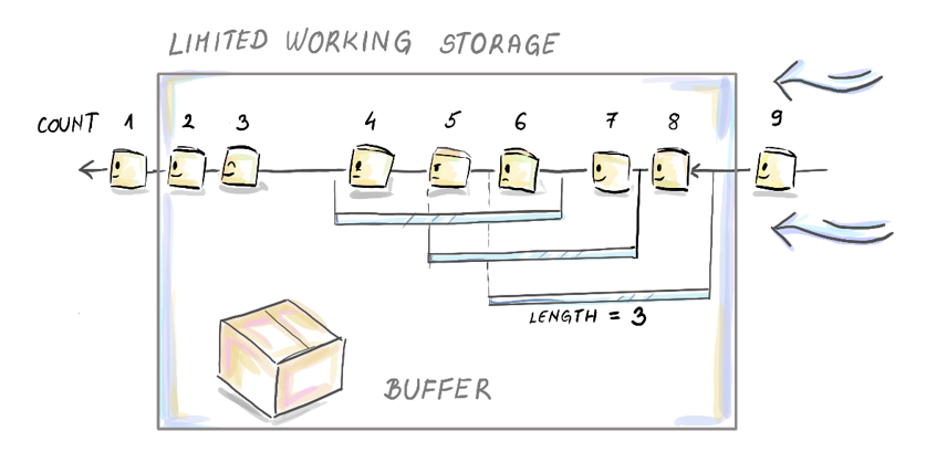
: Figure shows last three sliding movements by the count-based window. Notice that window length is not necessarily all that we can fit into our working storage, but that is definitely the maximum in history that we can cover. Hence in applications where we want “as much history as possible” to influence our data stream analysis one would extend the length of the window to “everything we can fit”. Keep in mind that aside from a sub-stream that we need to operate in one-pass mode we need to preserve space for our synopses and computation needed to build and update them. This is indicated by the buffer space show.
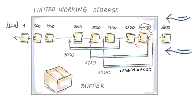
: Here we can see the time-based sliding window of length W=2000 ms and its three last sliding (meaningful w.r.t. to the arrival times of the data tuples) movements. We started the data stream at time 0 ms and at time 1 ms the first data tuple arrived. Then two more arrived at 500ms and 1000 ms. We are currently observing the stream after 5500ms. The three last movements of the window are indicated, that changed the content of the window: from 1400 to 1401 ms (data tuple arrived at 3400 ms enters the window), from 2700 ms to 2701 (notice that this movement resulted in 4 data tuples in the window) and from 2800 ms to 2801 ms (data tuple at 2800 ms is discarded).

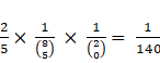
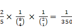
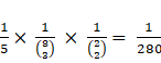
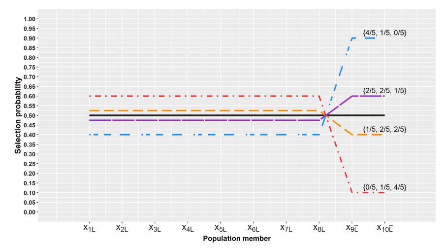
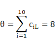
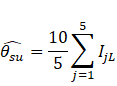
Graph shows selection probabilities for differently biased die from our example. The probabilities to draw a sample of type 3,4 and 5 are shown on each line that shows probability of selection for all . Notice how for any biased sampling strategy, via the three-sided biased die, the selection probabilities “move” away for 0.5. The drection of the “movement” depends on loyalty card existence with respect to the particular purchase . Our original biased die corresponds to the shift denoted by .

Summary
- Streaming data pipeline is a natural environment for showcasing the algorithms and data structures we learned so far and those we have yet to put under our belt.
- The combination of distributed computing and imperative of real-time delivery of results in streaming data applications create numerous opportunities for shortening the end-to-end latencies by smart use of hashing, bloom filters, count-min sketches and hyper log-logs.
- Tasks like joining large tables saved across a heterogeneous storage systems, de-duplication in the stream, monitoring network traffic and load balancing are all real examples of such opportunities.
- Real-time analytics is possible if stakeholders can agree on level of tolerance for latency in such systems. Data generating mechanism is prone to periodic or incidental changes and our streaming data algorithms should be able to accommodate and detect those in time. There are data stream models like count-based or time-based sliding windows to allow for recency adjustments to detect such phenomena known as concept shifts and concept drifts.
- Sampling is a powerful and long established technique for answering questions about an intractable set by systematically forming its subset and answering the same question from the subset. Long and well established theory for statistical inference from the unbiased or biased sample can be of a lot of help to decide on the sample size and choose an estimator for our query answer to guarantee accuracy and precision necessary for practical purposes.
FAQ
What is the streaming data model and how does it differ from a traditional database system?
In the streaming model, data arrives continuously and is processed on-the-fly using limited working storage. Most items are never stored (or only archived in slow, non-indexed storage), so both updates and query answers must be computed in one pass with small time and space. Traditional DBMSs emphasize exact answers over flexible time, while streaming emphasizes timely, approximate answers via synopses for both standing and ad-hoc queries.What are the main tiers of a streaming data pipeline and what does each tier do?
- Data collection: consolidates data from producers, performs initial transformation/augmentation.- Message queuing (brokers): buffers between producers and consumers, restores ordering/consistency, de-duplicates, balances load, prevents congestion and load shedding.
- Analysis tier: maintains synopses, runs continuous and ad-hoc queries, sampling, and estimation.
- Consumers/edge: dashboards, ad bidding, alerts, automated actions that use the real-time results.
Where do Bloom filters, Count-Min Sketch, and HyperLogLog fit in a streaming pipeline?
- Bloom filters: used for early filtering and de-duplication (e.g., in message queuing or collection), and to pre-prune joins across systems (Bloom-join).- Count-Min Sketch: monitors rates and detects heavy hitters for network traffic and broker load balancing using packet/message headers.
- HyperLogLog: estimates cardinalities (e.g., distinct IPs) efficiently; useful for network surveillance and analysis-tier metrics.
These synopses often work in sequence across tiers, not only inside the analysis tier.
What is a Bloom-join and why is it useful for hybrid warehouses (EDW + HDFS)?
A Bloom-join exchanges Bloom filters of the join key (e.g., IP address) between systems before the actual join. Each side filters its table using the other side’s Bloom filter, so only candidate rows are shuffled and sent. This two-way pre-filtering reduces network I/O and shuffle volume, speeding the final join while tolerating a controlled false positive rate.How is de-duplication implemented in streaming systems and what are the trade-offs?
Intercept/worker nodes persist message IDs in a fast store and maintain a Bloom filter of seen IDs. Incoming messages are checked; if the ID is reported present (with a small false positive rate), the duplicate is dropped before queuing. Trade-offs: a false positive can discard a legitimate message (e.g., a payment or critical event). Mitigations include idempotency keys, exactly-once processing guarantees, compensation workflows, and tuning the Bloom filter’s false positive rate.How does Count-Min Sketch help with network monitoring and load balancing?
CMS hashes flow identifiers (e.g., source/destination IP/port, protocol) or broker IDs and increments counters by packet size or queued requests. Periodic normalization yields rates; flows or brokers exceeding a threshold are flagged as heavy hitters/overloaded. CMS guarantees no underestimation, so sub-threshold items are safe; flagged items may include false positives and can be verified precisely on a small set.What do “one pass”, “small time”, and “small space” mean for streaming algorithms?
- One pass: each tuple is processed once as it arrives.- Small time: per-item update and query times are sublinear, ideally polylogarithmic in the size of the maintained sub-stream/synopses.
- Small space: synopses fit in limited working memory alongside any needed buffers. These constraints enable timely analytics despite high ingestion rates.
What are concept shift and concept drift, and why do they matter?
Concept shift is an abrupt change (e.g., sudden spikes in keywords during a disaster); concept drift is a gradual change over time. Both alter the data-generating process, so analytics that weight all history equally can become stale or misleading. Streaming systems counter this with time decay and windowing to emphasize recent data.What is the sliding window model and how do time-based and count-based windows differ?
The sliding window model restricts analysis to the most recent data:- Time-based: includes all tuples from the last W time units.
- Count-based: maintains the most recent W tuples.
Window length is chosen by application recency needs and bounded by available working memory (leaving room for synopses and updates). Larger windows capture more history; smaller windows react faster to shifts.

 Algorithms and Data Structures for Massive Datasets ebook for free
