4 Frequency Estimation and Count-Min Sketch
This chapter motivates frequency estimation in data-intensive systems such as bestseller lists, trending queries, IP traffic summaries, and anomaly detection, and explains why naive key–value counting becomes impractical when the number of distinct items is huge or when keys are pairs. In one-pass streaming with strict memory limits, exact top-k and heavy hitters require too much space; even the elegant majority-element algorithm does not generalize. To address this, the chapter turns to approximate methods and introduces the Count-Min Sketch (CMS), a compact probabilistic structure for estimating item frequencies and supporting heavy-hitter style analytics over massive streams.
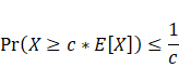
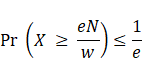
CMS represents counts in a d-by-w matrix of integer counters indexed by d independent hash functions. An update increments one counter per row; a query hashes the key in every row and returns the minimum of the d counters, producing an estimate that may overcount but never undercounts. Overestimation arises from collisions and is controlled by two parameters: epsilon (additive error as a fraction of the stream’s total count N) and delta (failure probability). With width w ≈ e/ε and depth d ≈ ln(1/δ), CMS guarantees fx ≤ fest ≤ fx + εN with probability at least 1 − δ. The sketch can power streaming top-k by pairing it with a min-heap of size k that tracks current leaders via CMS estimates, and its implementation is straightforward with fast hash functions.
Case studies underline the practicality: a smart-bed sensor app tracks user restlessness using CMS over user or (user, sensor) keys, and an NLP pipeline replaces a massive word–context co-occurrence matrix with a CMS plus small marginals for words and contexts, delivering over two orders of magnitude space savings while preserving PMI-based similarity quality. The chapter also extends CMS to approximate range-sum queries via dyadic intervals: maintain one sketch per dyadic level, update every range containing an arriving key, and answer a query by decomposing it into O(log n) dyadic ranges and summing their estimates, achieving logarithmic time and bounded error. Overall, CMS offers tunable error–space trade-offs and serves as a versatile building block for frequency estimation, heavy hitters, and range analytics on massive streaming datasets.
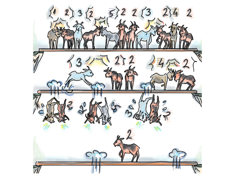
: We find a majority element in an array by having different neighboring elements throw each other out. In this example, after we throw out (1,2), (2,5), (3,2), and then (3,2) and (4,2), we are left with the majority element 2.
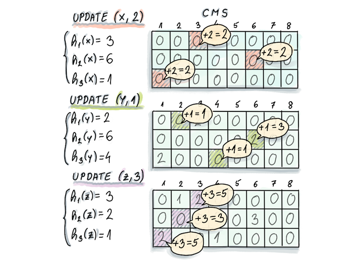
: Three update operations of x, y and z performed on an initially empty CMS of dimensions 3x8. Computed hashes indicate which columns in the respective rows of count-min sketch need to be updated.
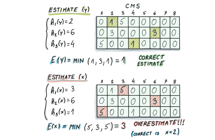
: Example of estimate operations on the count-min sketch from Figure 4.2. In the case of element y, whose true frequency is 1, count-min sketch reports the correct answer of 1 (the minimum of 1, 3 and 1). However, in the case of the element x, whose true frequency is 2, count-min sketch reports 3 (the minimum of 5, 3 and 5). Refer to the Figure 4.2 to convince yourself that during earlier update operations, y and z together incremented all the counters that are used by x, thus resulting in an overestimate for x.
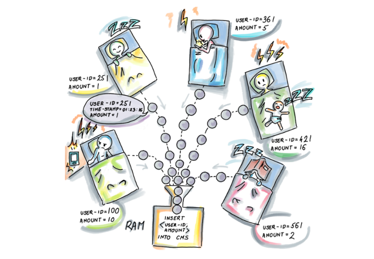
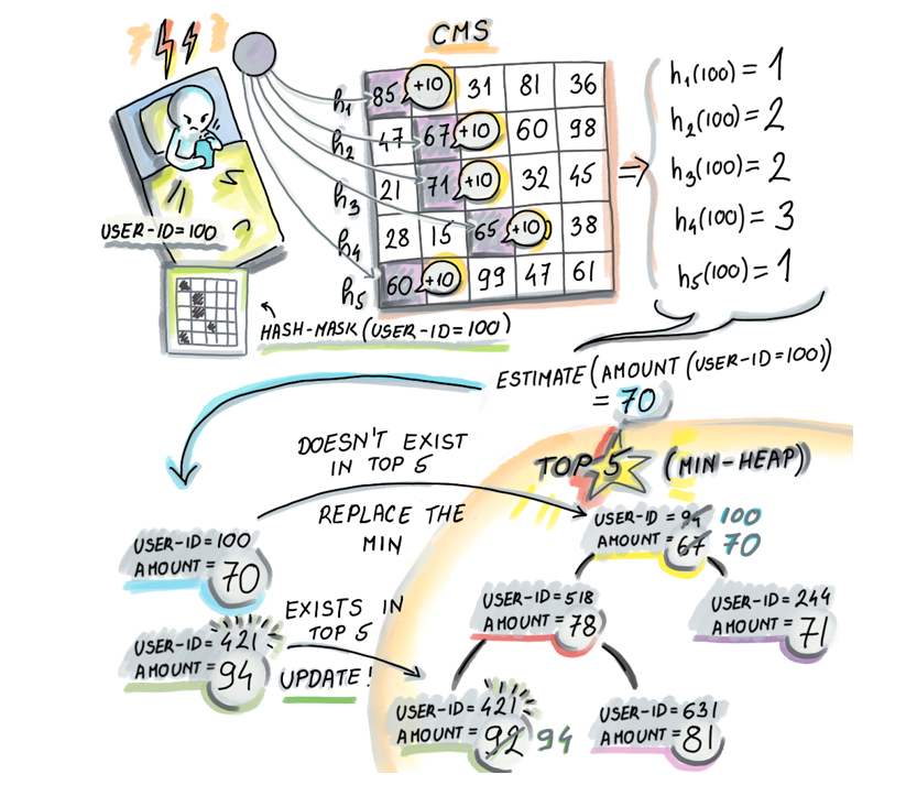
: All sleep data is sent to a central archive, but before that, input into count-min sketch residing in RAM for later analysis. The (user-id, amount) pair is used as the input for the data structure, where the frequency of user-id increases by amount. The key that is hashed is user-id.
: Using min-heap and count-min sketch together to find top-k restless sleepers. Every time the count-min sketch is updated with a (user-id, amount) pair, like with (100, 10) in this example, in order to maintain a correct list of top-k restless sleepers, we do an estimate on frequency of the recently updated user-id. In our case, the estimate for user-id 100 will be 70. Then, if the user-id is not present in the min-heap and it has a higher value than the min (as it does in our example), we will extract the min and insert the new (user-id, amount) pair into the min-heap. If the pair was already present, its amount needs to be updated by deleting and re-inserting the pair with the new updated (higher) amount.
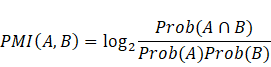
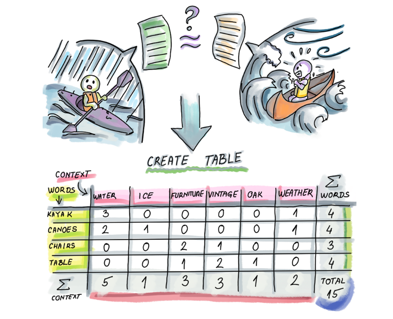
: To preprocess the text corpus for computing PMI, one way is to create a matrix M where the entry M[A][B] contains the number of times the word A appears in the context B. So for example, ‘kayak’ appears 3 times in the context of ‘water’ and 0 times in the context of ‘furniture’. We also produce the additional count for each word (the last column of the matrix), and count for each context (the last row in the matrix), as well as the total number of words (lower right corner).
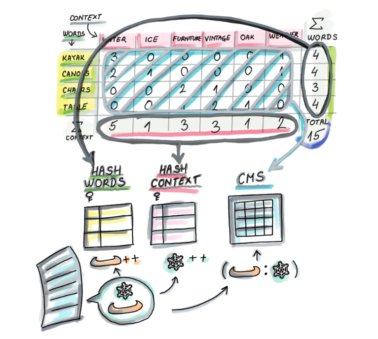
: The transformation of the matrix from Figure 4.6 to save space: the word-context pairs stored in the main body of the matrix are replaced by a count-min sketch that stores frequencies of word-context pairs. Because the number of distinct words (and contexts) is not that large, we can store each in their own hash table with the appropriate counts. In other words, when we encounter a new pair (word, context), we increment the count of the pair in the CMS, and also increment respective counts in the word hash table and the context hash table. To calculate the PMI for a word-context pair, we do the estimate query on the count-min sketch, and find the appropriate counts of the word and the context in the respective hash tables.


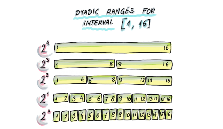
Dyadic ranges for the interval [1, 16]. Dyadic ranges of level 0 are the bottom-most with ranges of size 1, then the ranges of level 1 are the level above with the ranges of size 2, and in general dyadic ranges at level i are of size 2i. Dyadic ranges across different levels are mutually aligned.
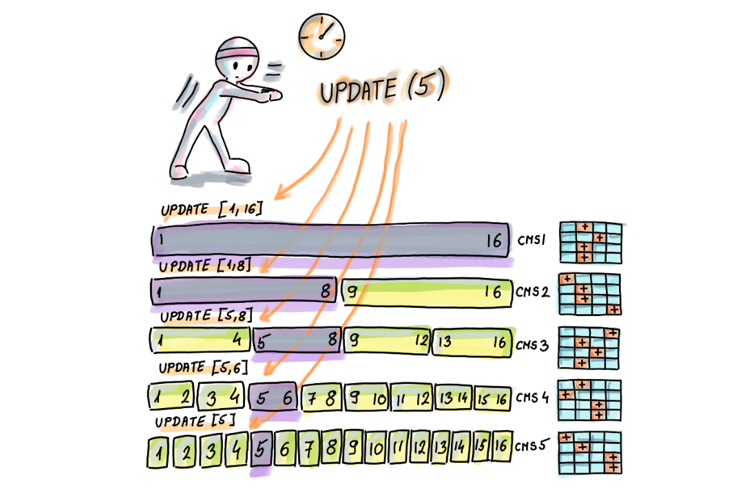
: An update of one element is transformed into one update per level. For example, if we update 5, we effectively update [1,16] in CMS1, [1,8] in CMS2, [5,8] in CMS3, [5,6] in CMS4, and [5] in CMS5. Instead of updating an element, we are updating a corresponding range to which the element belongs, in the relevant CMS.
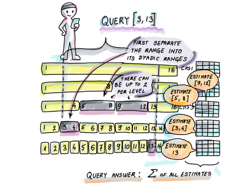
: In this example, the query range [3, 13] is separated into [3,4]∪[5,8]∪[9,12]∪[13], and we will obtain the frequency estimate for [3,13] by obtaining the frequency estimates for the mentioned ranges and summing them up.
Summary
- Frequency estimation problems arise very commonly in the analysis of big data, especially in sets that have many occurrences of very few items and a small number of occurrences of many items. Even though in the standard RAM setting, frequency estimation can be simply solved in linear-space, solving this problem becomes very challenging in the context of streaming data where we are allowed only one pass over the data and sublinear space.
- Count-min sketch is well suited to solve the approximate heavy hitters problem and many other problems in sensor and NLP domains.
- Count-Min sketch is very space-efficient and it has two error parameters,
 (controlling band of overestimate) and
 (controlling the failure probability) that are tunable and determine the dimensions of the count-min sketch. If the allowed band of overestimate error is kept as a fixed percentage of the total quantity of data N, then the amount of space in count-min sketch is independent of the dataset size.
- It is possible to do fairly accurate frequency estimates for range queries using count-min sketch by decomposing a range into a set of dyadic ranges, and using
 count-min sketches.
FAQ
What real-world problems motivate frequency estimation and the use of Count-Min Sketch (CMS)?
Popularity and anomaly detection tasks rely on counting how often items occur in high-rate streams: top-k searches, bestseller lists, frequent IP pairs, or sudden spikes in sensor readings. Storing exact per-item counts with a key–value dictionary can be infeasible when the number of distinct keys is huge (e.g., Zipf-like distributions or pair keys like (source,destination)), so CMS offers compact approximate frequency estimates.What is the heavy hitters problem and why is it hard to solve exactly in one pass?
Given N items and a parameter k, heavy hitters are items with frequency > N/k. In a strict streaming model (one pass, sublinear space), maintaining exact counts for many potential candidates can require linear space in the number of distinct items, which is often impractical. Hence we use approximate methods that trade small error for large space savings.How does the Boyer–Moore majority vote algorithm differ from general heavy hitter detection?
Boyer–Moore finds a majority element (frequency > ⌊N/2⌋) in one pass using O(1) extra space by canceling mismatches. This elegance does not extend to general heavy hitters (e.g., N/k for k>2), where multiple candidates must be tracked, pushing space toward linear if we demand exact answers.What is Count-Min Sketch and how do its update and estimate operations work?
CMS is a d×w array of counters with d independent hash functions. On update(item, c): for each row j, increment CMS[j][hj(item)] by c. On estimate(item): return the minimum across rows of CMS[j][hj(item)]. Collisions can add extra counts, so estimates can overestimate but never underestimate the true frequency.What error guarantees does CMS provide and how do I configure its size?
With parameters ε (additive overestimate as a fraction of total count N) and δ (failure probability), CMS guarantees for every item x: true_fx ≤ estimate(x) ≤ true_fx + εN with probability ≥ 1−δ. Configure width w ≈ e/ε and depth d ≈ ln(1/δ). Space is w·d counters; time per update/estimate is O(d).What are the main limitations of CMS’s error model?
The additive error is proportional to the total stream count N, not to an item’s own frequency. Thus small-frequency items can experience large relative error. Also, overestimates arise from hash collisions; although multiple rows reduce the chance of consistent collisions, the error band εN still applies.How can I maintain the top-k items with CMS?
Combine CMS with a min-heap of size k. For each stream update: (1) update the CMS, (2) estimate the item’s frequency, (3) if it exceeds the heap’s minimum (or the item is already in the heap), adjust the heap accordingly. This keeps approximate top-k using O(k) extra space plus the CMS.How is CMS used in practice (e.g., sensors and NLP)?
- Sensor app: Use (user-id, amount) updates to track restlessness per user; a min-heap + CMS gives top-k restless sleepers in near real time with small memory.- NLP PMI: Replace the huge word–context count matrix with a CMS for pair counts, while keeping marginal word/context counts in small hash tables. This drastically reduces memory with minimal impact on PMI quality.

 Algorithms and Data Structures for Massive Datasets ebook for free
