11 Learning representations: LeCun, Bengio, Hinton, and the rise of deep learning

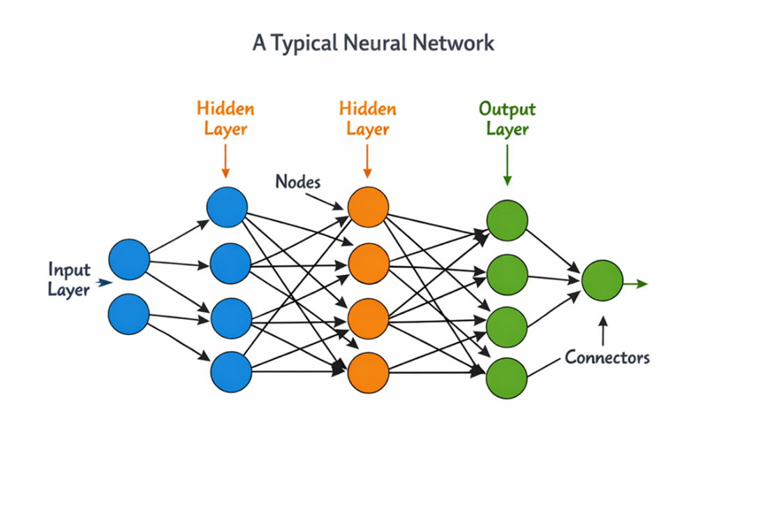
A simplified feedforward neural network containing an input layer, two hidden layers, and an output layer. Information moves forward through weighted connections to produce a prediction. During training, error information moves backward so that the weights and biases can be adjusted. Modern deep networks typically contain many hidden layers and many nodes within each layer, producing millions or even billions of adjustable parameters. Despite that scale, they follow the same basic forward-and-backward process shown here.

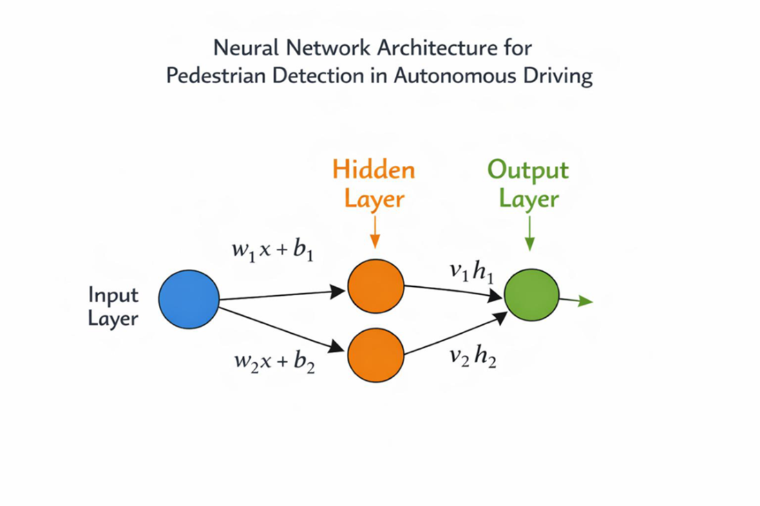
The compact feedforward neural network used in the pedestrian-detection example. The input 𝑥 is transformed at the hidden nodes using weights 𝑤1 and 𝑤2 and biases 𝑏1 and 𝑏2. After activation, the resulting hidden outputs ℎ1 and ℎ2 are weighted by 𝑣1 and 𝑣2 and combined at the output node. The output node then adds its own bias, not shown, and applies a final activation function to produce the predicted probability.

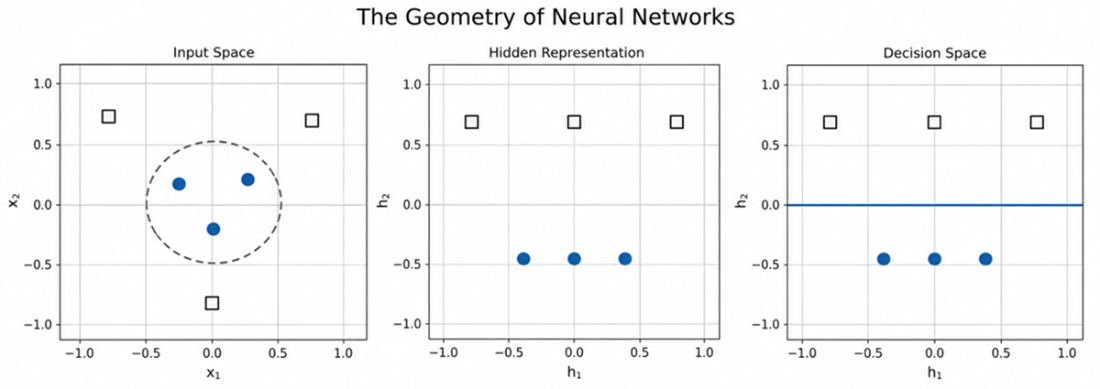
A nonlinear transformation reorganizes the same six observations so that classes requiring a curved boundary in the input space can be separated by a straight boundary in the learned representation.

• LeCun, Bengio, and Hinton’s 2015 synthesis marked the emergence of deep learning—and the multilayer neural networks that make it possible—as the dominant learning method in artificial intelligence, including applications in vision, speech, and language. Neural networks had existed for decades, but larger data sets, greater computing power, improved training methods, and representation learning finally allowed their theoretical promise to translate into reliable performance at scale.
• A neural network produces a prediction by passing inputs forward through layers of nodes connected by weights and biases. Activation functions introduce the nonlinearity needed to represent relationships that successive linear transformations alone cannot capture. Depth determines how many transformations are composed, while width determines how many patterns a layer can represent at the same stage of processing.
• Neural networks can produce class probabilities or continuous numerical predictions. In classification, the predicted probability, thresholded class, and resulting action are distinct: the network first produces a probability under its current parameters, and a predetermined threshold converts that probability into a class or operational response. In regression, the continuous prediction is used directly without a classification threshold. In both cases, training evaluates the continuous output through a loss function because it preserves information that would be lost by reducing the prediction immediately to a discrete decision.
• A loss function converts the discrepancy between a network’s prediction and the observed outcome into a continuous value. Cross-entropy serves this role for classification, while squared-error loss is widely used for regression. Backpropagation applies the chain rule in reverse through the network to calculate how each weight and bias influenced the loss. Gradient descent then uses those gradients and a selected learning rate to update the parameters incrementally across observations, mini-batches, and epochs.
• Neural-network learning brings several earlier foundations together. Minimizing cross-entropy is equivalent to maximizing the likelihood of the observed classes, connecting training to Fisher. The same loss can be interpreted through Shannon as the information cost of assigning probabilities that do not align with observed outcomes. Bayesian neural networks extend fixed-parameter networks by representing parameter uncertainty, while MacKay showed how inference, information, regularization, and model evidence could be interpreted within a common learning framework.
• Width provides capacity to represent many patterns in parallel, while depth allows those patterns to be combined into progressively more structured representations. Because hidden layers learn nonlinear transformations, observations requiring a complicated boundary in the original input space can become easier to separate in the learned representation. The value of that transformation depends on whether it also organizes unseen observations in ways that support accurate prediction.
• Greater capacity does not guarantee generalization and can instead allow a network to learn noise or training-specific details. Architectural and hyperparameter choices establish the available capacity before training, while validation and test data evaluate whether performance carries beyond it. Weight decay, dropout, early stopping, and data augmentation constrain how capacity is used, continuing the generalization objective pursued through different mechanisms by support vector machines and random forests.
• High average accuracy does not by itself establish that a neural network is reliable. Data quality, coverage, representativeness, distribution shift, and bias affect neural networks as they affect other machine-learning methods, while scale can make learned dependencies more difficult to identify. Calibration, stability under changing inputs, interpretability, computational requirements, and production monitoring must also be considered before a network’s probabilities and classifications can be trusted operationally.
• After 2015, self-supervised learning reduced dependence on manually labeled data, while multimodal and foundation models expanded the kinds of information and tasks one system could accommodate. Transformers then changed how relationships could be represented and provide the next architectural step. Later, scaling experiments showed that coordinated increases in data, parameters, and computation could produce predictable performance gains.

FAQ