3 Forecasting with TimeGPT

This chapter introduces TimeGPT as a practical, foundation-model approach to time series forecasting, contrasting it with the challenges of training bespoke models from scratch. Using a multi-store Walmart weekly sales dataset with rich exogenous drivers as a running example, it frames how a single, pretrained generative model can forecast diverse series, quantify uncertainty, and even repurpose its forecasts for anomaly detection. The narrative emphasizes hands-on use—zero-shot forecasting, fine-tuning, leveraging external variables, robust evaluation, and long-horizon scenarios—while highlighting when these capabilities help and where they may fall short.

TimeGPT is a full encoder–decoder Transformer, pretrained on a vast, multi-domain corpus to learn varied temporal patterns and generalize across frequencies and scales. It is probabilistic, producing prediction intervals via conformal prediction adapted to time series, and it natively accepts exogenous features—provided both their past and future values are available. Accessed through a simple API client, it delivers strong zero-shot baselines, and can be specialized with lightweight fine-tuning by setting the number of steps, the optimization loss, and the breadth of parameters to update, which often yields measurable gains. For extended horizons, a variant tuned for long-range dependencies improves accuracy over the base model.

The chapter also covers practicalities: preparing data with the expected identifiers and timestamps, building future exogenous inputs, and interpreting forecasts with Shapley-based feature contributions. It recommends cross-validation with non-overlapping windows to obtain reliable metrics, and shows how anomaly detection is performed by labeling points that fall outside high-confidence historical forecast intervals—while noting limitations at the series start and the precision–recall trade-off controlled by interval width. Overall, TimeGPT streamlines modern forecasting through an API-first workflow that combines rapid zero-shot use, targeted fine-tuning, principled uncertainty, explainability, and basic anomaly detection across a wide range of series and horizons.

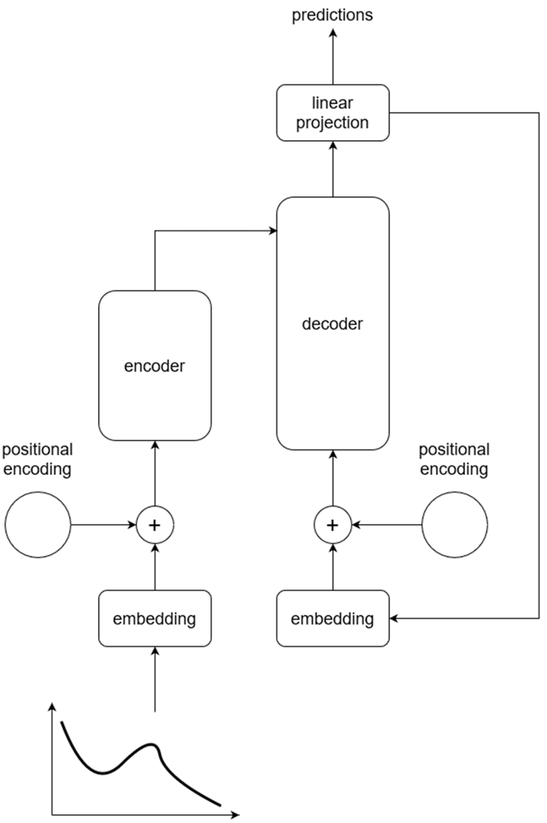
Overall architecture of the Transformer model. Notice how the output of the decoder is sent back as an input to continue generating the output sequence.

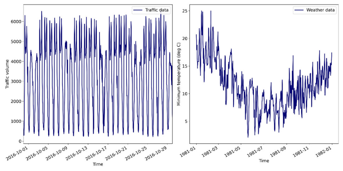
Different temporal patterns appear with different domains. On the left, hourly traffic data shows a daily and weekly seasonality. On the right, daily temperature data exhibits a yearly seasonality.

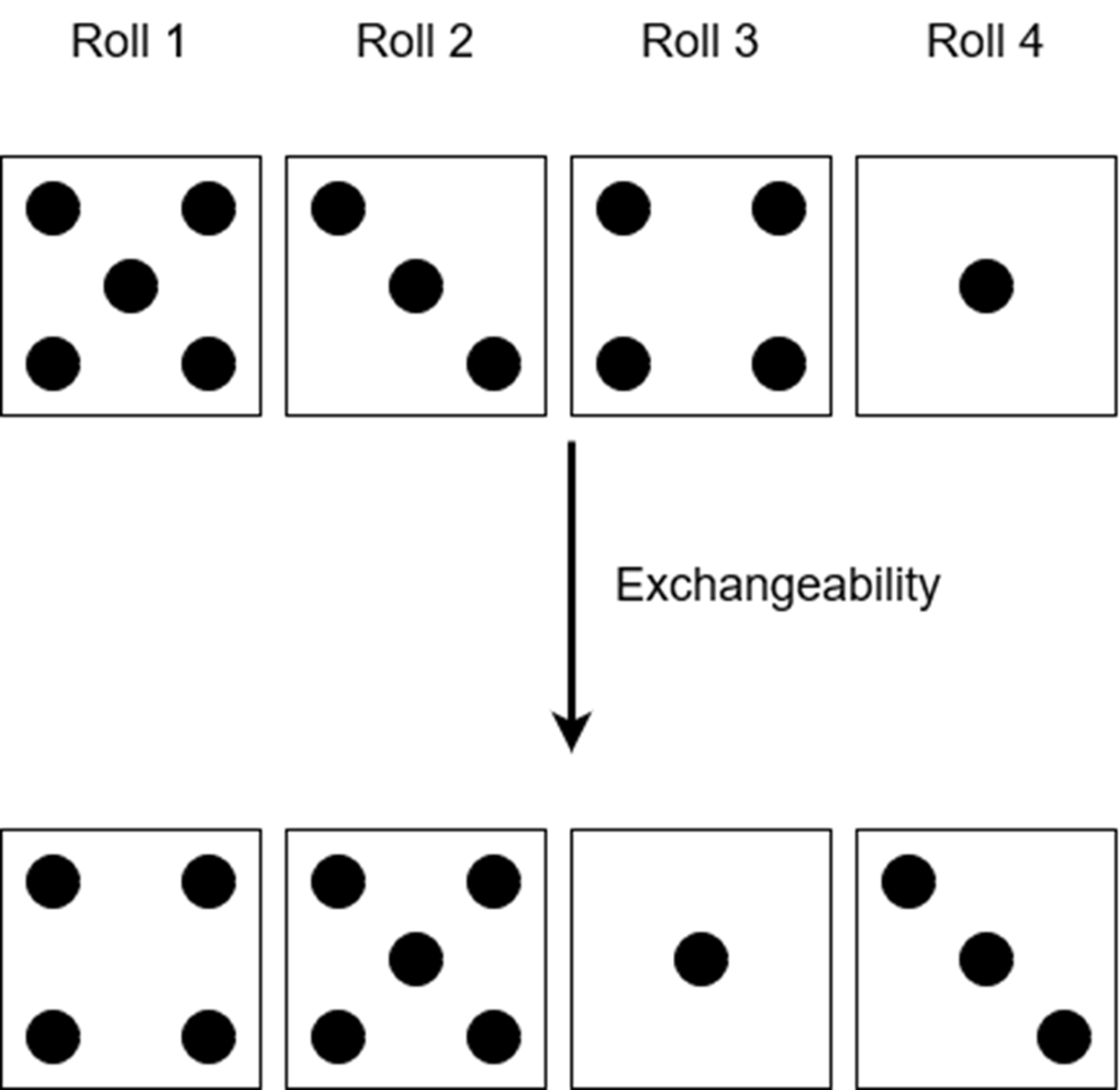
Rolling a die is an example of exchangeability. Here the die is rolled four times. Rearranging the obtained values gives a sequence that is equally likely as the original one.

Overview of conformal prediction for time series data. Historical predictions are used to calculate conformity scores. These scores are then used to generate a range of possible values for each point forecast. From that range of possible values, we calculate the quantiles corresponding to a user-specified confidence level.

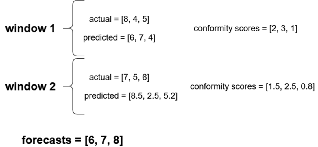
Guiding example to build conformal prediction intervals. Here, we suppose we run cross-validation using two windows and a horizon of three time steps. For each window, we have the actual and predicted values. The forecasts represent predictions for the future, for which we do not know the actual values. The goal is to build the conformal prediction interval for each point forecast.

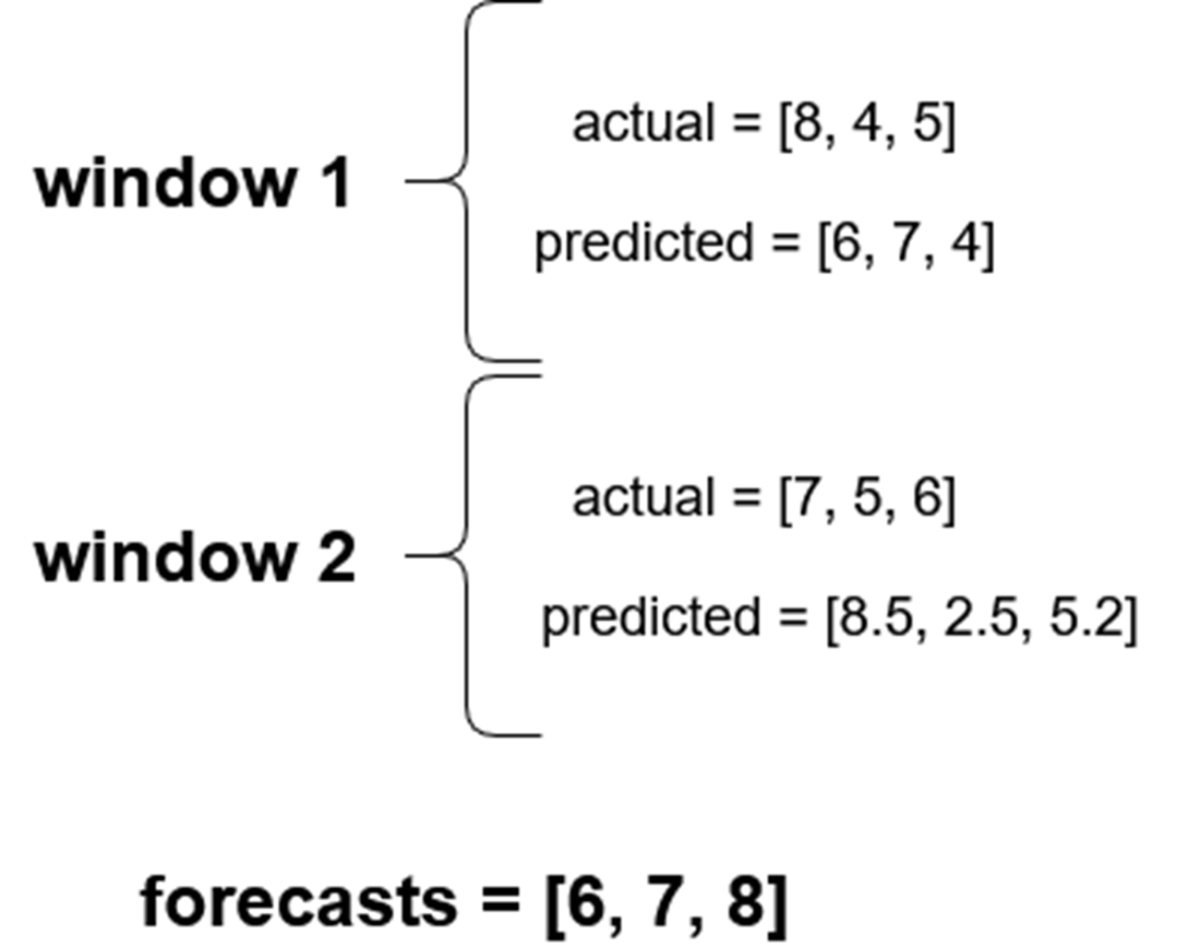
Adding conformity scores for each window. Here, the conformity score is calculated as the absolute difference between the actual and predicted value.

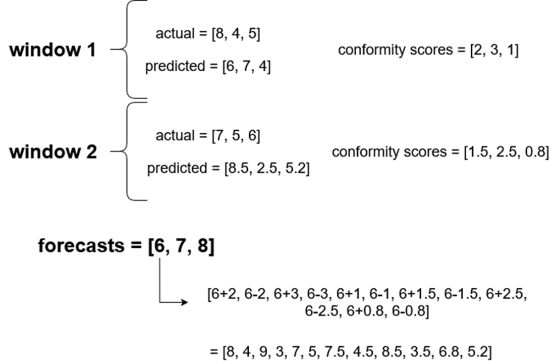
Calculating the range of possible values for the first point forecast. Notice that we simply add and subtract all conformity scores from the forecast to get its range of possible values. The same step is repeated for each point forecast.

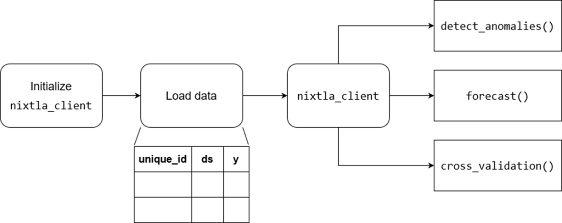
General workflow of TimeGPT. After initializing the client and loading the data, we then use the client for anomaly detection, forecasting and cross-validation.

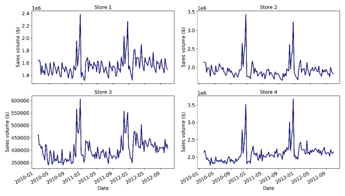
Plotting the weekly sales of four Walmart stores. While each store shares a similar general pattern, the granular behavior is unique for each store.

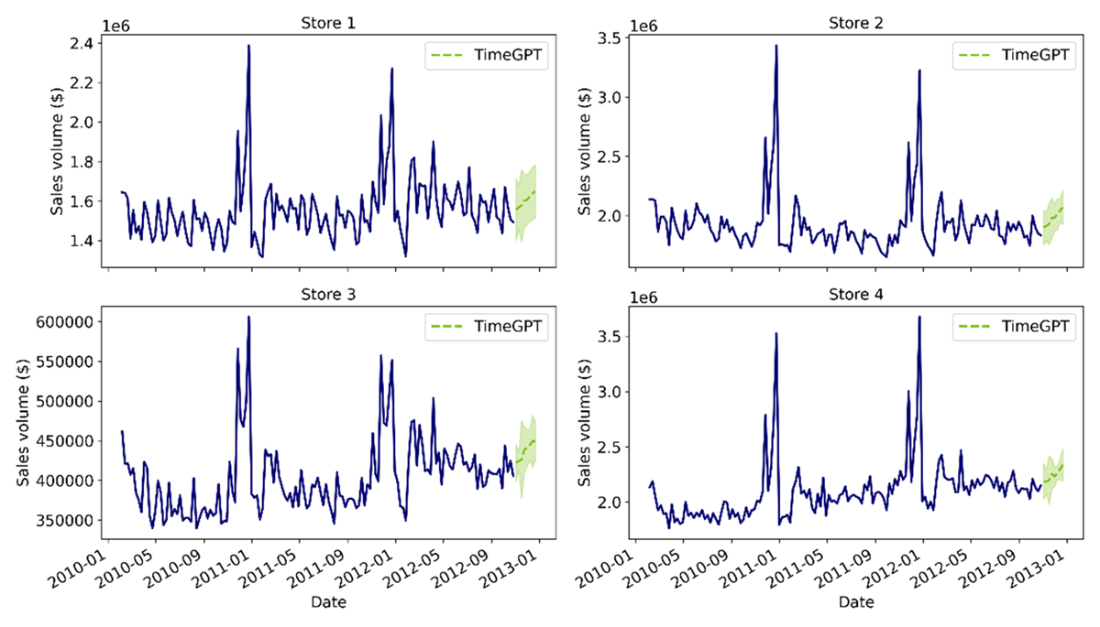
Plotting the predictions obtained with TimeGPT. Notice how the prediction intervals are different for each series.

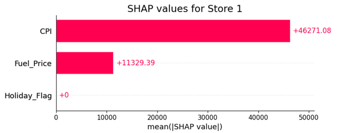
Average Shapley values of exogenous variables for predicting the weekly sales of a Walmart store. On average, the CPI feature increases the base forecast by 46271 and fuel price increases it by 11329 on average. Holidays have no impact on the final value.

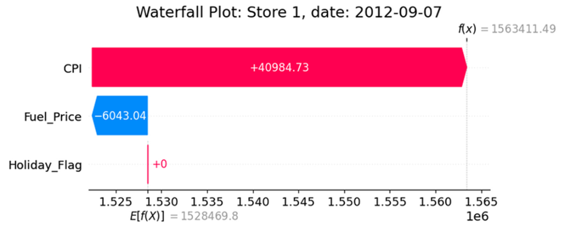
Waterfall plot for the prediction on 2012-09-07. The base value of 1528469.8 is the forecast if no exogenous features were used. Then, the value of fuel price at that date decreases the prediction by 6043.04. However, the value of CPI then increases it by 40984.73, which results in a final prediction of 1563411.49.

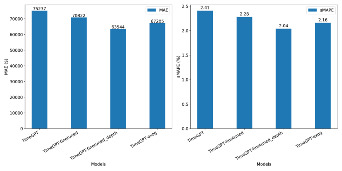
Plotting the performance of zero-shot forecasting, fine-tuning, and fine-tuning with exogenous variables. Lowest values indicate the best performance. Here, fine-tuning more parameters, without using features, results in the best performance.

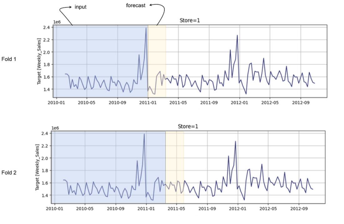
Illustrating the behavior of cross-validation with TimeGPT. A fold designates one round of cross-validation. By default, non-overlapping windows are used.

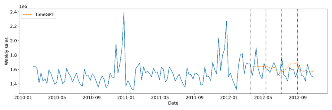
Visualizing cross-validation in TimeGPT. Each vertical line indicates the start of a cross-validation window or fold. There are four of them, which corresponds to the number of windows set in listing 3.19. In between each vertical line, we see the predictions being made at each fold. The prediction line (dashed) is hard to see as it mostly overlaps the actual data.

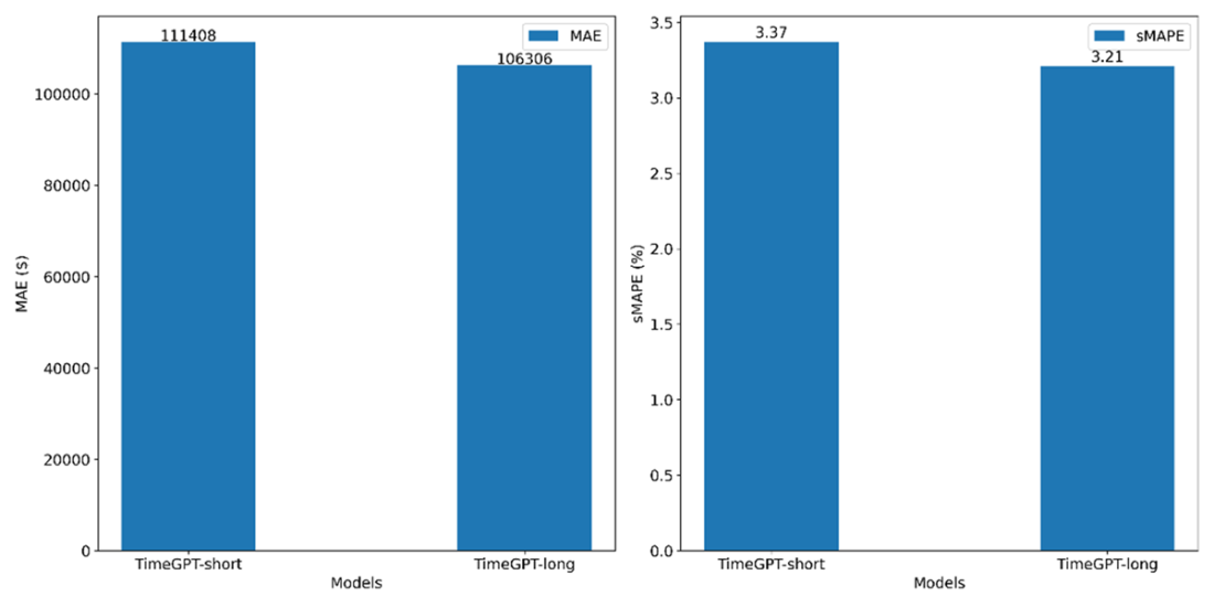
Comparing the performance of the base model and timegpt-1-long-horizon. Lower values are better. Here, when forecasting on a long horizon, using the adapted model generated better results.

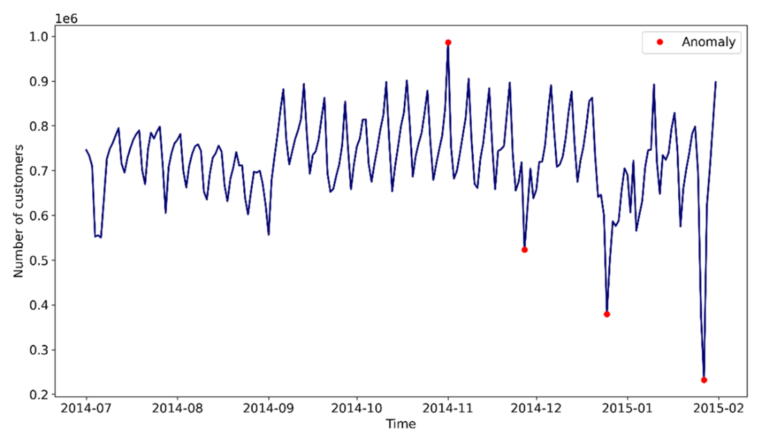
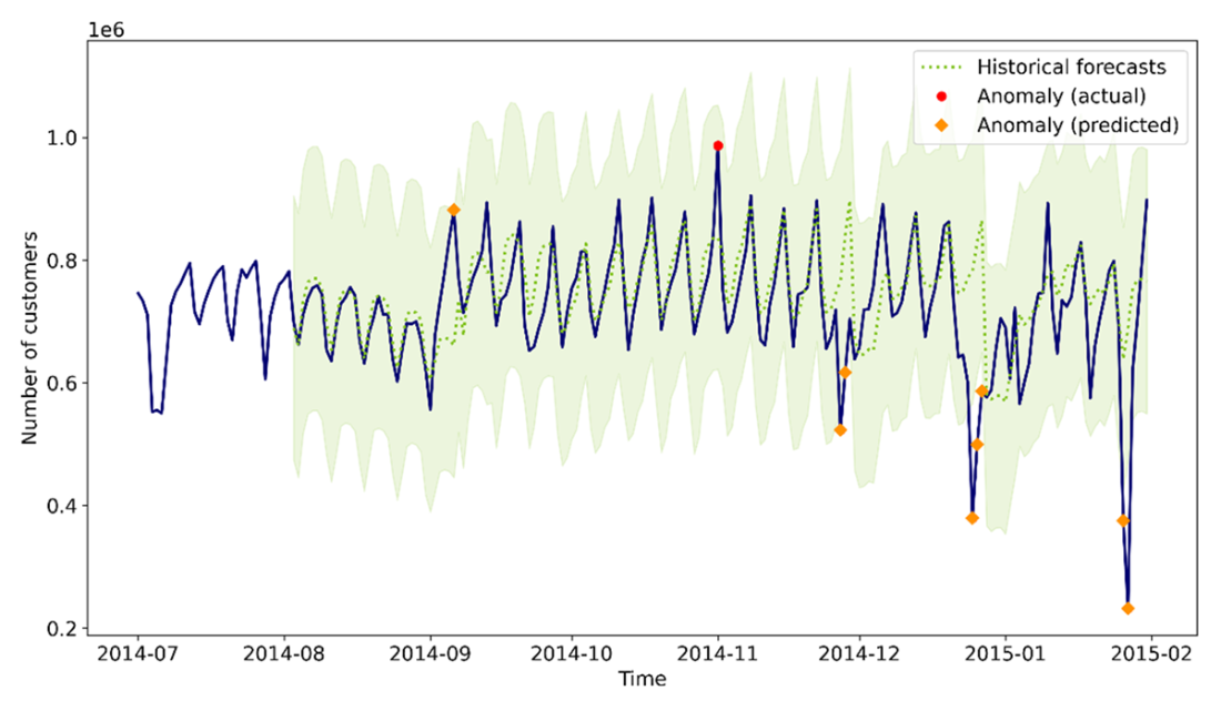
Daily number of taxi customers in New York city, from July 2014 to the end of January 2015. The four dots represent the anomalous points.

Plotting the anomalies detected by TimeGPT. The dotted line shows the historical forecasts. The shaded area represents the 99% prediction interval. If a point falls outside the interval, it is labelled as an anomaly. Diamonds indicate predicted anomalies while dots represent the actual anomalies not detected by TimeGPT. If a detected and an actual anomaly coincides, meaning that the model correctly identified the anomaly, then only a diamond is shown.

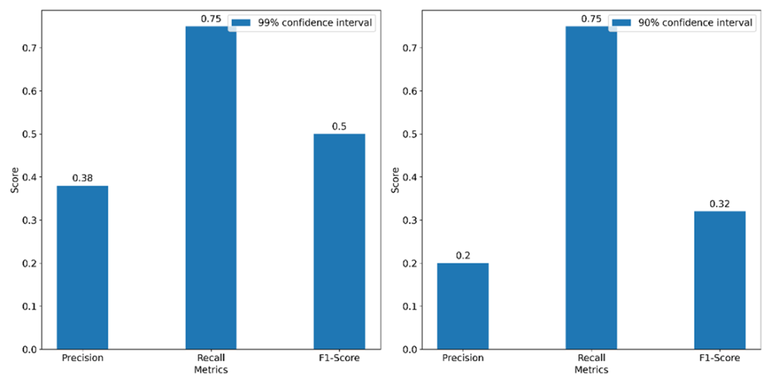
Comparing the performance of anomaly detection using different prediction intervals. Higher values are better. The 99% prediction interval results in more balanced results, as the F1-score is higher than when we reduce the prediction interval.

• TimeGPT is a proprietary model developed by Nixtla. It is a pretrained generative Transformer trained on 100 billion data points.
• TimeGPT is accessed via API and requires an access token.
• With TimeGPT, we can perform zero-shot forecasting, forecast multiple series concurrently, fine-tune the model, include exogenous variables, do cross-validation and detect anomalies.
• When fine-tuning, we can specify the number of steps and the loss function to be used.
• When forecasting on a long horizon, remember to use the model timegpt-1-long-horizon.
• When doing anomaly detection, a smaller level, or a smaller prediction interval, results in more anomalies being detected, so the recall increases and the precision decreases. The opposite is true when the prediction interval is large.

FAQ