6 The Birth of Hyperscale

The chapter explains how modern AI entered the hyperscale era: not through a single new architecture, but through the discovery that larger models, larger datasets, and larger compute budgets produce surprisingly predictable improvements. The jump from GPT-2 to GPT-3 made this visible to the public, showing that a decoder-only Transformer scaled from 1.5 billion to 175 billion parameters could gain abilities such as in-context learning without major architectural redesign. Kaplan’s 2020 scaling laws gave researchers a practical roadmap, showing that loss falls smoothly with more parameters, data, and compute, even though returns diminish. This turned progress into an allocation problem: decide how much compute should go into model size, data, and training time.

The chapter also stresses that scaling is not magic or inevitability. Later work, especially DeepMind’s Chinchilla results, showed that many frontier models had been too large for the amount of data they received, shifting attention toward better token-to-parameter balance and far larger training corpora. Post-Chinchilla experiments then tested the limits of that insight, with models trained on far more tokens per parameter than earlier rules suggested. At the same time, the chapter complicates the idea of smooth progress: training loss may decline predictably, but downstream capabilities are jagged. Benchmarks can make abilities look sudden, contaminated datasets can inflate results, and some tasks even show inverse scaling before improving again. Scaling laws are therefore useful planning tools, not guarantees of reliable intelligence.

The final part shows that hyperscale depended on engineering as much as theory. Data parallelism worked while models fit on a single device, but larger networks required model parallelism, tensor sharding, memory sharding, and pipeline scheduling. GPipe demonstrated how micro-batch pipeline parallelism could spread models across accelerators, reduce memory pressure, and enable much larger vision and translation systems. Later approaches such as Megatron-LM and ZeRO improved on this by slicing computations within layers and eliminating redundant memory storage across devices. The chapter’s broader lesson is that the smooth curves of scaling laws were made real only through difficult systems work: keeping thousands of accelerators busy, coordinating communication, managing memory, and surviving long, failure-prone training runs.

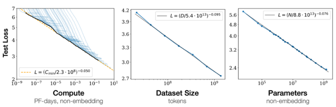
Language modeling performance improves smoothly as model size, dataset size, and amount of compute used for training increase. For optimal performance, all three factors must be scaled up in tandem. Empirical performance has a power-law relationship with each factor when it isn’t bottlenecked by the other two. Used with permission granted by a coauthor (Ben Cross).

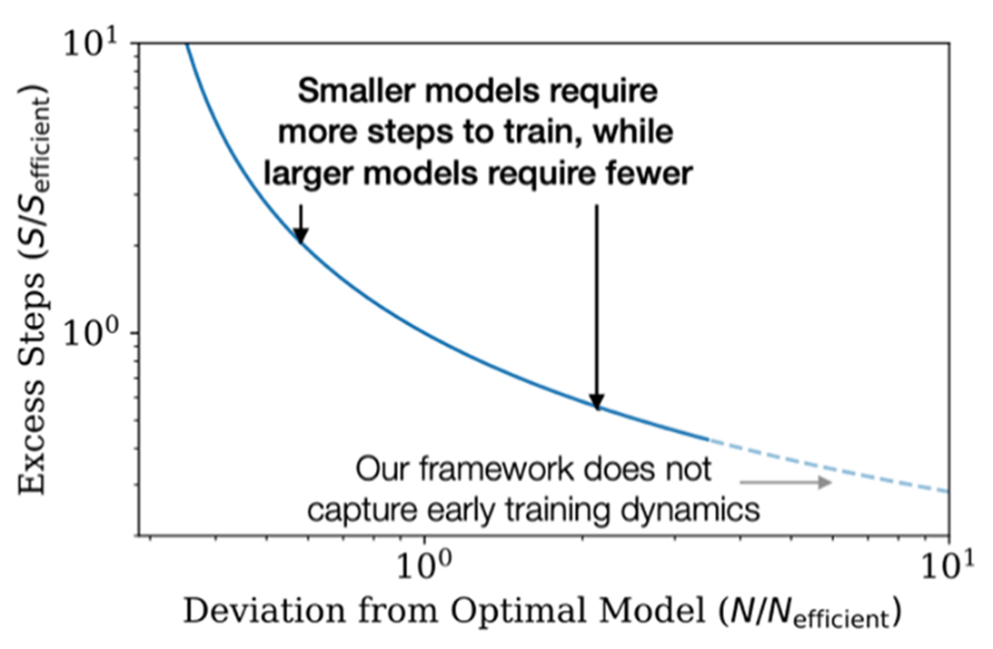
Models larger than the compute-efficient size require fewer training steps, potentially enabling faster training if sufficient additional parallelism is possible. Used with explicit permission granted by a co-author (Ben Cross).

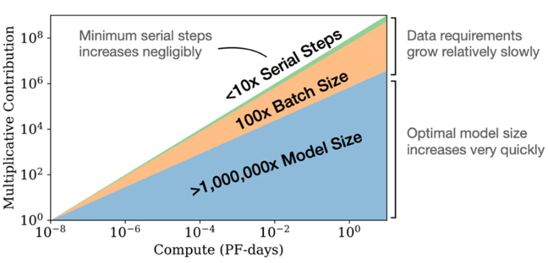
The authors illustrate how to allocate training resources given a billion-fold increase in compute. For optimal compute-efficient training, most of the increase should go toward expanding model size. Only a relatively small increase in data is needed to prevent reuse. Of the additional data, most can be used to increase parallelism by using larger batch sizes, requiring only a minimal increase in serial training time. Used with explicit permission granted by a coauthor (Ben Cross).

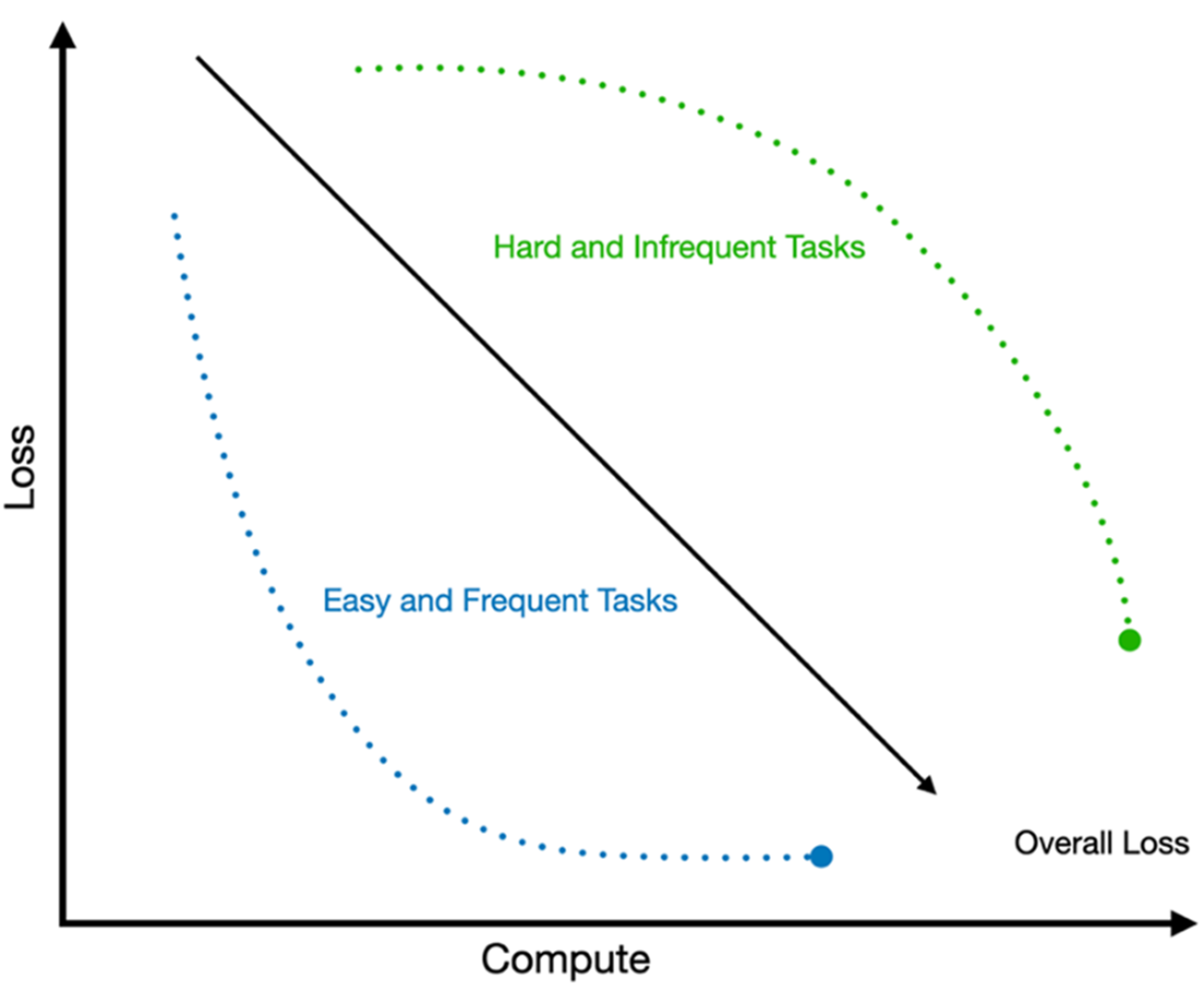
A model will learn some tasks more easily than others. Easy tasks are frequent with dense data, while hard tasks are infrequent with sparse data.

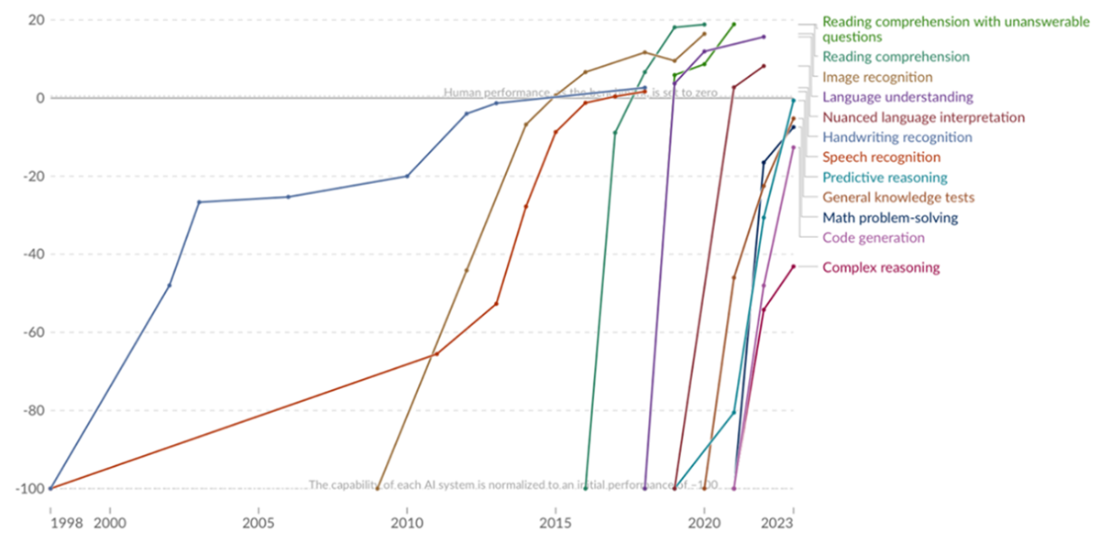
Line chart (1998–2023) showing multiple series that rise steeply after 2018 toward the “human performance = 0” line for reading comprehension, code generation, math problem-solving, and complex reasoning, indicating rapid benchmark saturation.[59]

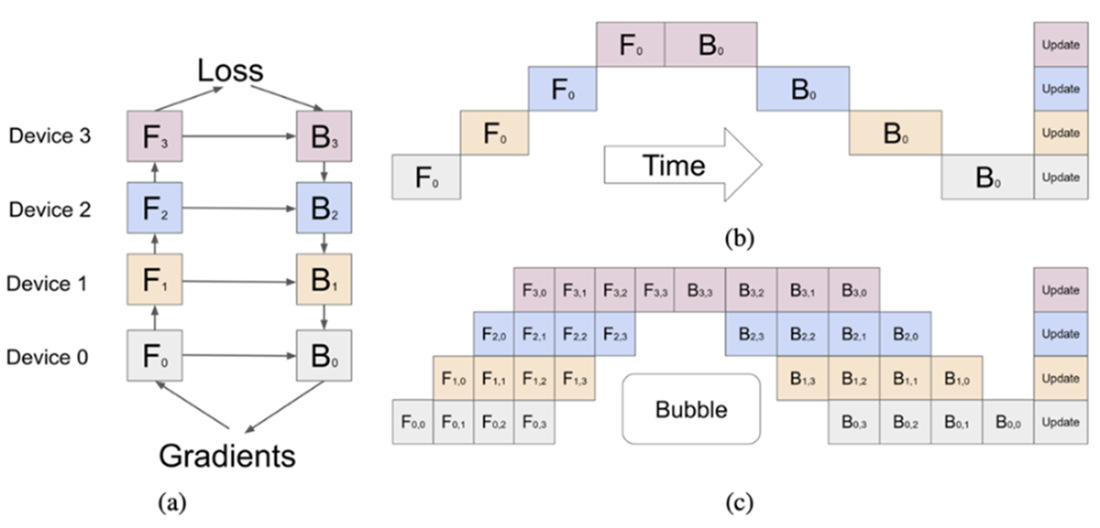
Pipeline parallelism compared to naive model parallelism. (a) A simple neural network partitioned across four accelerators, with forward passes 𝐹0 – 𝐹3 flowing upward and backward passes 𝐵0 – 𝐵3 flowing downward to compute gradients. (b) In naive model parallelism, layers are split sequentially across devices. Because each stage must wait for the previous stage to complete, much of the hardware remains idle, leading to low utilization. (c) Pipeline parallelism mitigates this inefficiency by splitting each mini-batch into smaller micro-batches. These micro-batches flow through the pipeline in a staggered fashion, keeping devices busy by processing different micro-batches simultaneously. While idle-time bubbles still appear during the pipeline “fill” and “drain” phases, overall utilization improves significantly. Gradients are accumulated across micro-batches, and updates are applied synchronously at the end of each full batch. Used with explicit permission granted by the lead author (Yanping Huang).

FAQ