2 The AlexNet Moment
The text explains how AlexNet became a turning point in artificial intelligence by proving that deep convolutional neural networks could outperform the dominant computer vision methods of the early 2010s. Before 2012, neural networks were widely viewed with skepticism: they were considered slow, hard to train, theoretically messy, prone to overfitting, and inferior to carefully engineered feature pipelines. The field favored methods such as SIFT, HOG, bag-of-visual-words, Deformable Parts Models, and SVMs, which relied on human-designed visual features. AlexNet’s dramatic ImageNet victory, reducing top-5 error from roughly 26% to about 15%, showed that learned representations could beat handcrafted features at scale.
The chapter situates AlexNet’s success within a broader shift involving data, compute, and optimization. ImageNet, built under Fei-Fei Li’s leadership, provided a dataset large and diverse enough for neural networks to learn useful visual hierarchies, even though early ImageNet competitions were still dominated by traditional feature engineering. At the same time, researchers such as Geoffrey Hinton, Yann LeCun, Yoshua Bengio, James Martens, and Ilya Sutskever helped keep neural network research alive during years of doubt. Martens’s work on training deep networks from scratch influenced Sutskever’s confidence that depth was not the real obstacle; better optimization, initialization, activations, and computational tools could make deep learning practical.
AlexNet succeeded because Krizhevsky, Sutskever, and Hinton combined several engineering and algorithmic choices into one scalable system. Its convolutional layers learned hierarchical visual features directly from pixels, while ReLU activations improved gradient flow, dropout reduced overfitting, data augmentation expanded the effective training set, careful initialization stabilized learning, momentum improved optimization, and two GPUs made the model feasible to train. The impact was immediate: by 2013, ImageNet competitors rapidly adopted CNNs, later architectures such as VGGNet, GoogLeNet, and ResNet pushed results further, and major technology companies began investing heavily in deep learning. AlexNet did not merely win a benchmark; it changed the field’s assumptions about what neural networks could do.
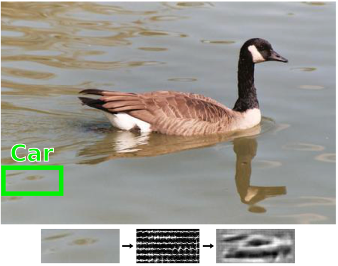
This figure shows a goose swimming (top), where an object detector mistakenly labels a small patch of rippled water as a car. Below the image are three visualizations that clarify the source of this error: a close-up of the water patch (left), the corresponding HOG features (middle), and a specialized visualization (right) showing that the rippled water’s features resemble those associated with cars in HOG feature space. Vondrick et al. (2013), figure 2.1. Used with express permission granted by the lead author (Carl Vondrick).
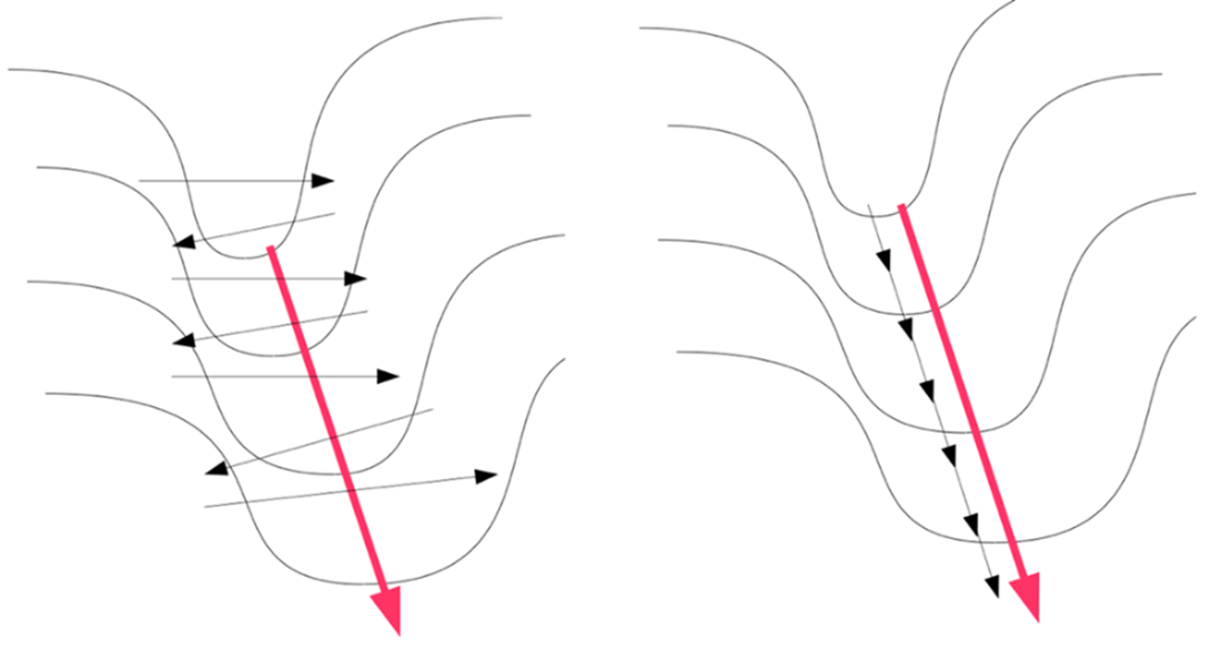
This figure illustrates the challenge of optimizing functions shaped like long, narrow valleys. The contour lines represent a valley, with the optimal direction of progress indicated by an arrow running along the valley’s base. Smaller arrows represent steps taken by gradient descent: the left diagram shows large steps oscillating inefficiently across the valley, while the right diagram shows small steps making slow progress along the base. The “pathological” nature does not arise from high or low curvature, but from the combination of high curvature across the valley and low curvature along it. Martens (2010), figure 1. Used with explicit permission granted by the author (James Martens).
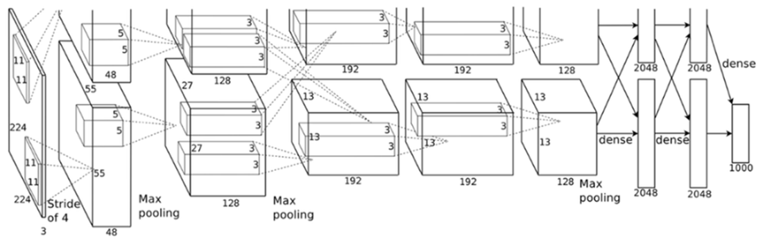
The AlexNet architecture (cropped in the original paper). The numbers indicate spatial dimensions and channel depth at each stage. The input image (224×224×3 RGB) passes through a series of convolutional and pooling layers that progressively reduce spatial resolution (224→55→27→13) while increasing channel depth (48→128→192→256). Early downsampling is driven by the first convolutional layer (11×11 filters with a stride of 4), followed by max pooling layers (3×3 windows with a stride of 2) that further reduce spatial dimensions. The stride determines how far a filter moves across the input at each step, controlling how densely the image is sampled and how quickly spatial resolution is reduced. Filter sizes (11, 5, 3) are depicted as cubes and define the local receptive field of each convolution. The two horizontal streams reflect the model’s original two-GPU training setup, where feature maps were split across devices (e.g., 48 + 48 = 96 channels). The fully connected layers (4096 neurons, implemented as 2048 + 2048 across GPUs) feed into a 1000-way output for ImageNet classification. Used with explicit permission granted by the lead author (Alex Krizhevsky).
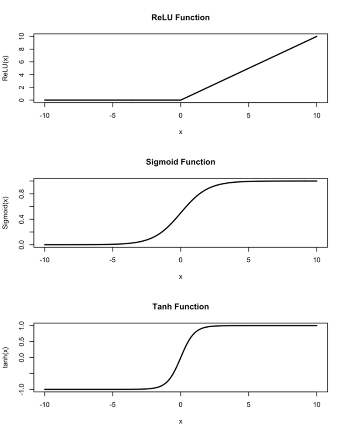
Plot of ReLU (top), sigmoid (middle), and tanh (bottom) activation functions generated in R by the author. Activation functions map input values (on the x-axis) to output values (on the y-axis). For example, ReLU produces zero for negative inputs; for positive inputs, the output equals the input (x < 0 and linear for x ≥ 0). The sigmoid function maps inputs to values between 0 and 1, resembling an S-curve. Similarly, the tanh function provides a smooth S-shaped curve but maps inputs to values between -1 and 1, centered at 0.
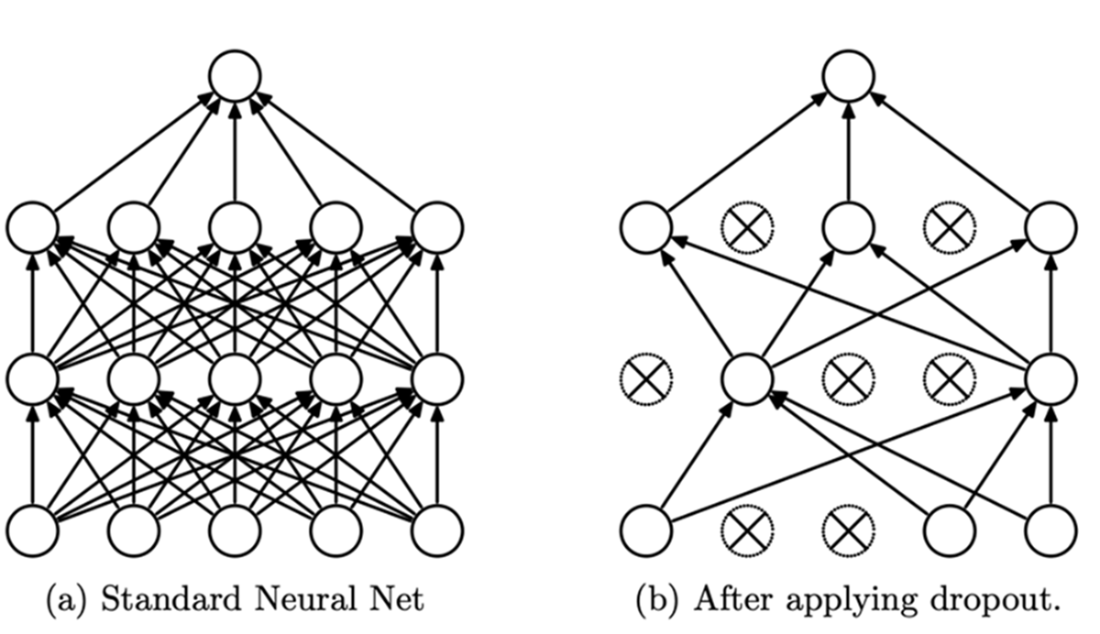
(Left) A standard neural network with two hidden layers. (Right) An example of a network produced by applying dropout to the network on the left. Used with explicit permission granted by the lead author (Nitish Srivastava).
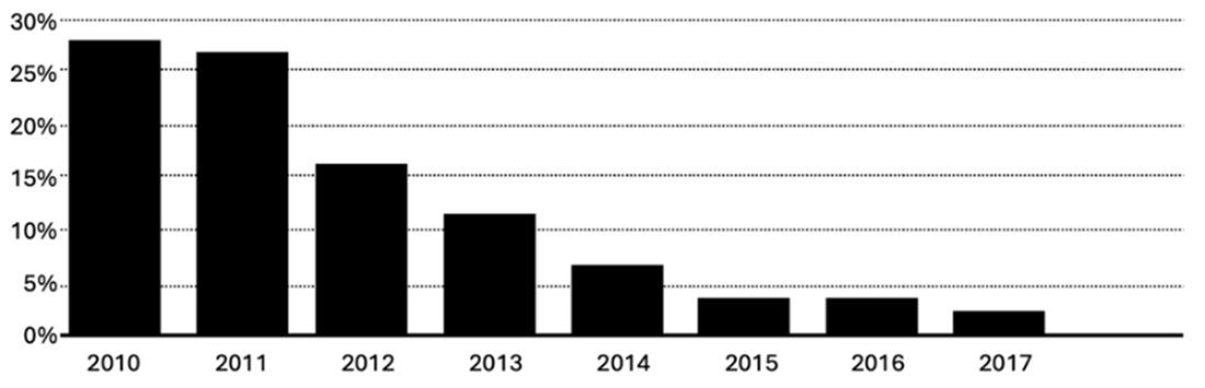
The top-5 error rates in the ILSVRC from 2010 to 2017. SIFT and SVM won in 2010 and 2011, but performance plateaued. CNNs won from 2012 to 2017, including AlexNet in 2012, and eventually saturated the benchmark.
FAQ
What was the “AlexNet Moment”?
The “AlexNet Moment” refers to the 2012 breakthrough when Alex Krizhevsky, Ilya Sutskever, and Geoffrey Hinton trained a deep convolutional neural network that dramatically outperformed traditional computer vision systems in the ImageNet Large Scale Visual Recognition Challenge. AlexNet achieved a top-5 error rate of about 15%, compared with roughly 26% for the best conventional handcrafted-feature methods.
Why was AlexNet’s ImageNet result so surprising?
Before AlexNet, many researchers believed artificial neural networks were impractical for serious computer vision tasks. The dominant systems used handcrafted features such as SIFT, SURF, HOG, bag-of-visual-words models, and SVM classifiers. AlexNet showed that a neural network trained end-to-end could learn better visual representations directly from data, overturning years of skepticism.
What does “top-5 error rate” mean?
Top-5 error rate measures how often the correct label is not among a model’s five most confident predictions. AlexNet’s roughly 15% top-5 error rate meant that the correct ImageNet category appeared in its top five guesses more than 84% of the time.
Why were artificial neural networks dismissed before AlexNet?
Artificial neural networks had gone through earlier waves of enthusiasm followed by disappointment. By the late 1990s and 2000s, they were often viewed as slow, hard-to-train black boxes that lacked strong theoretical guarantees. They suffered from problems such as overfitting, vanishing and exploding gradients, poor local minima, limited data, and insufficient computing power.
What was feature engineering, and why did AlexNet disrupt it?
Feature engineering was the practice of manually designing visual descriptors that captured useful image patterns. Methods such as SIFT, SURF, HOG, and Deformable Parts Models encoded human assumptions about edges, shapes, scale, and rotation. AlexNet disrupted this paradigm by learning hierarchical features automatically from raw pixels, allowing the model to discover representations rather than relying on hand-designed ones.
Why was ImageNet so important to AlexNet’s success?
ImageNet provided the scale needed for a large neural network to learn useful visual features. In 2012, the ImageNet-1k challenge used about 1.2 million images across 1,000 categories, far larger than benchmarks such as PASCAL VOC, MNIST, CIFAR-10, or the German Traffic Sign dataset. This large and diverse dataset gave AlexNet enough examples to train a deep model effectively.
How did AlexNet differ from earlier computer vision systems?
Earlier systems usually combined handcrafted image descriptors with shallow classifiers such as SVMs. AlexNet instead used a deep convolutional neural network with five convolutional layers followed by three fully connected layers. Its convolutional layers learned progressively more complex visual features, from edges and textures to object parts, while the fully connected layers converted those features into category predictions.
What technical innovations helped AlexNet train successfully?
AlexNet succeeded because several techniques worked together: ReLU activations improved gradient flow and sped up training, dropout reduced overfitting, data augmentation expanded the effective training set, careful weight and bias initialization stabilized learning, mini-batch stochastic gradient descent with momentum improved optimization, and two GPUs made the large model computationally feasible.
Why was ReLU important in AlexNet?
ReLU, or rectified linear unit, maps negative inputs to zero and leaves positive inputs unchanged. Unlike sigmoid or tanh activations, ReLU avoids saturation for positive values and helps gradients propagate through deeper networks. In AlexNet, switching from tanh to ReLU accelerated convergence by a factor of six and made it practical to train a much larger neural network.
What impact did AlexNet have after 2012?
AlexNet rapidly changed the direction of AI research and industry. In 2013, nearly all serious ImageNet competitors used convolutional neural networks, and by later years CNNs dominated the benchmark. The breakthrough also pushed major technology companies to invest heavily in deep learning, helped launch new AI labs and startups, and shifted public perception of neural networks from speculative curiosities to the foundation of modern AI.

 Sutskever's List ebook for free