7 Grover’s search algorithm

This chapter introduces Grover’s search as a practical example of the hybrid quantum–classical workflow for solving classical problems on a quantum computer. It frames unstructured search as finding any n-bit input x such that a deterministic function f(x)=1, with access only through an oracle, and motivates why many tasks (notably constraint satisfaction) can be reduced to this model. The chapter emphasizes an end-to-end mindset: classical preprocessing to build the problem instance, a quantum subroutine to gain speedup, and classical post-processing to validate or iterate, with later chapters applying and benchmarking the approach on richer problems.

The core abstraction is the quantum oracle. Two forms are used: marking oracles, which act on n+1 qubits and flip a target qubit when f(x)=1, and phase oracles, which act on n qubits and multiply marked basis states by −1. Because algorithms typically need phase oracles while implementations are often easier as marking oracles, the chapter shows how to convert between them via phase kickback. It provides compact Qiskit and Q# patterns to build marking oracles for “marked-list” functions, to realize phase oracles with a single auxiliary qubit, and to unit test them: compare matrices for phase oracles (diagonal ±1) and compare action against a classical function for marking oracles. These pieces set up the building blocks required by Grover’s search.

Grover’s algorithm prepares an equal superposition over the search space (“mean”), then repeats two reflections: a phase flip of the solutions (the oracle) and a reflection about the mean (the “diffusion” step). Geometrically, each iteration rotates the state toward the solutions by 2θ, where sin θ=√(M/N). The success probability rises, peaks, then oscillates, so the iteration count matters: the optimal number is about (π/4)√(N/M). If M is unknown, simple heuristics (e.g., doubling the iteration count across runs) work well, and results should be verified classically since Grover is probabilistic. Compared with random classical querying (≈N/M checks), Grover achieves a quadratic asymptotic speedup (≈√(N/M) oracle calls). The chapter gives Qiskit and Q# implementations that assemble the iteration from a phase oracle and the mean-preparation operator, outlines end-to-end testing (including deterministic cases like M/N=1/4 with one iteration), and tees up applications (such as N queens) and performance analysis in subsequent chapters.

Solving a classical problem on a quantum computer involves converting the problem to its “quantum” formulation, implementing the quantum algorithm as code, and evaluating the performance of the quantum solution to compare it to that of the classical algorithms for solving the same problem.

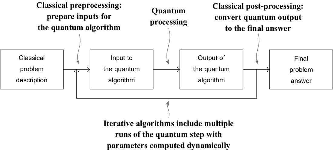
A quantum algorithm can combine classical and quantum computations. Typically, it starts with a classical data preprocessing step that prepares input data for the quantum computation and passes it to the quantum subroutine. The results of the quantum computation are then fed into another classical step, post-processing, that converts them into the final problem solution. Some of these steps can be omitted for simple algorithms or repeated with some variation for iterative algorithms.

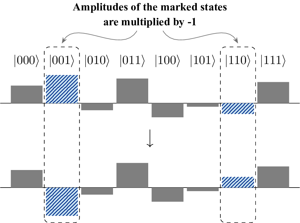
The effect of the phase oracle for the function that marks values \(001\) and \(110\) on a superposition state with real amplitudes. The amplitudes of the basis states that correspond to the marked values (striped bars) are multiplied by \(-1\). The rest of the amplitudes do not change.

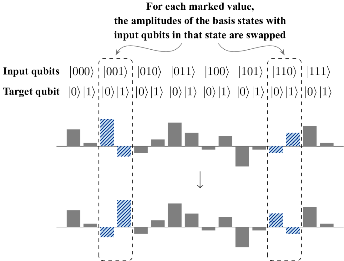
The effect of the marking oracle for the function that marks values \(001\) and \(110\) on a superposition state with real amplitudes. For each marked value, there are two basis states with the input qubits in the corresponding state (marked with striped bars): for one of them, the target qubit is in the \(\ket{0}\) state, and for the other one — in the \(\ket{1}\) state. The amplitudes of these pairs of basis states are swapped. The rest of the amplitudes do not change.

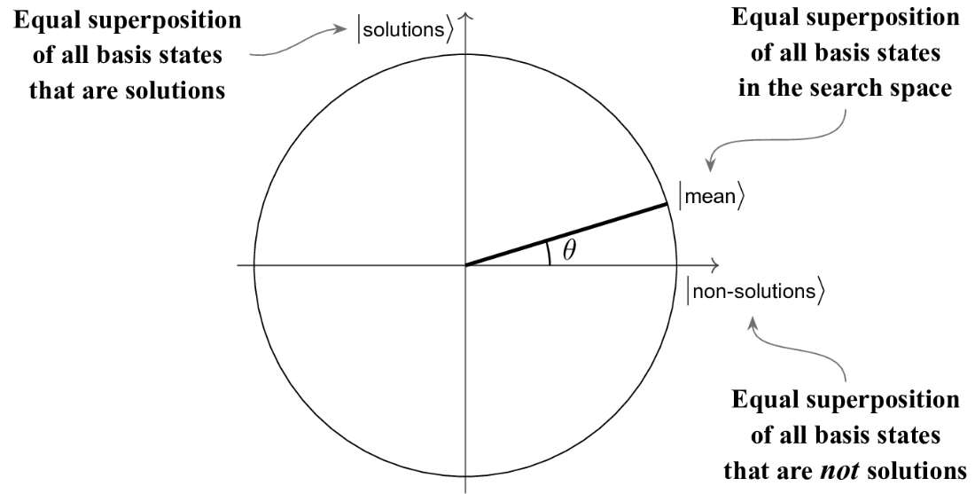
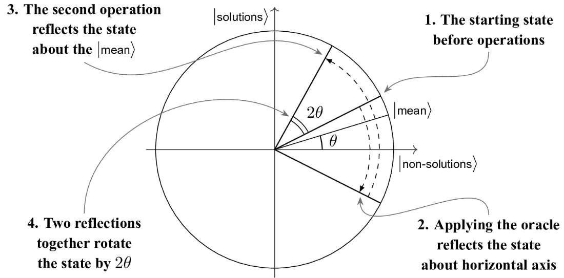
The main states used in Grover’s search algorithm. \(\ket{\textrm{mean}}\) is the superposition of all basis states in the search space (that is, states that correspond to bit strings that are potential solutions to the problem). These bit strings can be split in two groups: the ones that are solutions (included in the superposition \(\ket{\textrm{solutions}}\)) and the ones that are not (\(\ket{\textrm{non-solutions}}\)). The angle \(\theta\) is defined by the number of problem solutions and the size of the search space.

The main operations used in Grover’s search algorithm. Applying the phase oracle reflects the system state about the horizontal axis, the average of all non-solutions. “Reflection about the mean” reflects the system state about the mean state, the average of all states in the search space. Together, these two operations rotate the state of the system counterclockwise by a fixed angle.

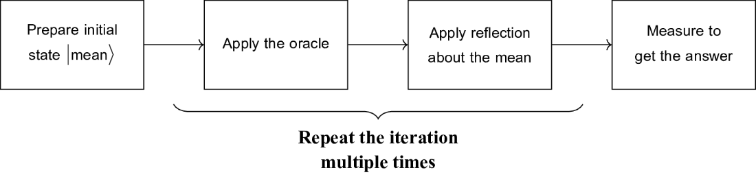
The overall structure of Grover’s search algorithm. You start by preparing the system in the mean state, the average of all states in the search space. Then you apply several iterations, each composed of applying the phase oracle followed by a reflection about the mean. Finally, you measure the system and check whether the result is an answer to the problem.

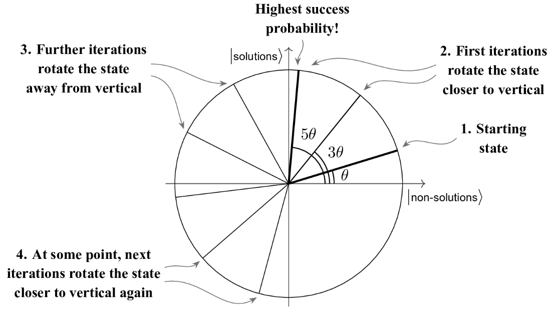
Each iteration of Grover’s algorithm rotates the state of the system in counterclockwise direction by the angle \(2\theta\). Up to a certain point, each iteration rotates the state closer to the vertical axis, the \(\ket{\textrm{solutions}}\) state. The closer the state is to \(\ket{\textrm{solutions}}\), the higher the probability of the measurement yielding a correct answer is. If you apply too many iterations (in this case, three or more), the state will go beyond vertical, and further iterations will decrease success probability.

• Programs that utilize quantum algorithms are often hybrid: they combine quantum computations with classical preprocessing for preparing the inputs to the quantum subroutine and post-processing for interpreting its outputs and producing the final answer or making decisions about the next computation to run.
• Unstructured search problem gives you a deterministic function that converts an input bit string into a single bit \(0\) or \(1\). Your goal is to find an input \(x_0\) for which the value of the function \(f(x_0) = 1\).
• An oracle is a tool that allows you to calculate the function for any given input but does not expose any information about the internal implementation of that function. Oracles are used in both classical and quantum computing to discuss generic algorithms that do not depend on the specific problem instance.
• Phase oracles encode the values of the functions in the signs of amplitudes of the input basis states.
• Marking oracles encode the values of the functions in the state of an additional qubit.
• You can convert a marking oracle into a phase oracle and vice versa using variants of the phase kickback trick.
• Grover’s search algorithm can solve the unstructured search problem for a function given as a quantum oracle. It offers a quadratic speedup in the number of queries to the quantum oracle compared to the “bruteforce” classical algorithm that has access to the function only via a classical oracle.
• Grover’s algorithm is a probabilistic algorithm; it produces the correct result with high probability, but not in \(100%\) of cases. You need to validate the answer \(x_0\) it gives you by calculating the value \(f(x_0)\) using a classical computation and checking that it is indeed \(1\).

FAQ