6 Evaluate classical functions on a quantum computer
This chapter explains how to solve classical problems on a quantum computer by turning classical computations into reversible ones and then implementing them as quantum programs. It outlines the end-to-end workflow: reformulate the classical task in “quantum” terms, implement the resulting algorithm (often as a hybrid of quantum and classical steps), test its correctness, and finally evaluate performance against the best classical methods. As a running theme, the chapter focuses on search problems—especially Boolean satisfiability—as a clear, widely applicable example, and introduces reversible computing as the essential bridge between classical functions and unitary quantum operations.
The core technique is to embed any classical function f(x) into a reversible transformation that preserves the input and writes the result into a separate bit: (x, y) → (x, y xor f(x)). This resolves the fundamental constraint that quantum gates must be reversible, while still enabling evaluation on superpositions by linearity. The chapter starts with single-bit functions to motivate correct and incorrect approaches (in-place works only for reversible functions), then builds a practical library of Boolean operations as quantum circuits: NOT via X, XOR via CNOT, AND via Toffoli (multi-controlled X), and OR via De Morgan’s law using controlled-on-zero variants of X; multi-input AND/OR follow from multi-controlled gates. It connects this construction to a synthesis pipeline: decompose a high-level function into Boolean primitives, make each primitive reversible, and map the reversible network to quantum gates.
Because intermediate results must not be left entangled with the rest of the system, the chapter emphasizes ancilla management and uncomputation (Bennett’s trick): compute the result, copy it to the final output, and then uncompute to return all ancillas to |0>. This is applied to evaluating Boolean expressions in conjunctive normal form: allocate ancillas to hold clause values, compute each clause (handling negated literals with temporary X gates), combine them with a multi-controlled AND into the output, and uncompute the clauses. A concrete testing strategy verifies correctness on basis states by comparing with classical results, ensuring the output matches f(x) and the inputs are preserved; examples in Qiskit use statevector inspection, while Q# tests use CheckAllZero and the within–apply (conjugation) pattern to automate uncomputation. Together, these methods provide a systematic path from classical specifications to correct, testable quantum implementations, setting up the oracles needed for algorithms like Grover’s search.
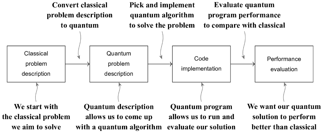
To solve a classical problem on a quantum computer, we start by converting the problem to its “quantum” formulation to which we can apply a quantum algorithm. After this, we implement the algorithm itself as a quantum program. Finally, we evaluate the performance of the quantum program and compare it to that of the best classical algorithm for solving the same problem. This way, we can see whether this quantum algorithm offers a practical advantage over the classical approaches.
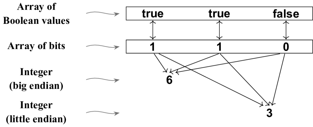
The inputs and outputs to any function can be represented in several equivalent ways. An array of Boolean values true and false is the same as an array of bits \(0\) and \(1\), which can then be interpreted as a binary notation of an integer. For integers, make sure to track whether the notation you use is big endian (most significant bit stored first) or little endian (least significant bit stored first)!
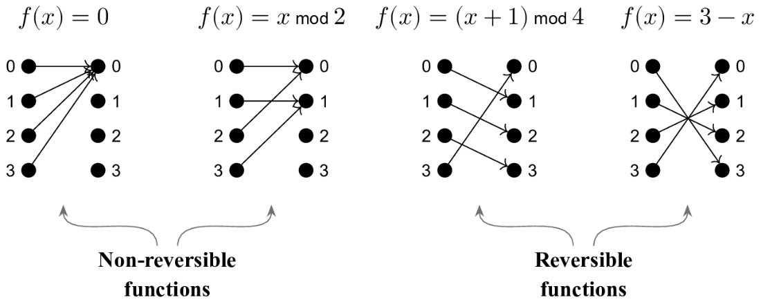
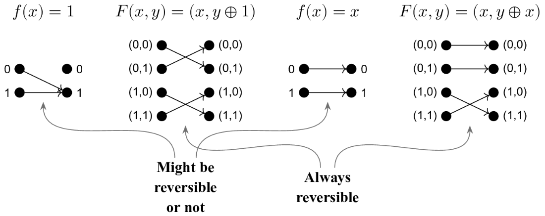
A classical function is reversible if it converts each input to exactly one output, and each output is produced by exactly one input. In other words, the input that produced a certain output can be restored from that output.
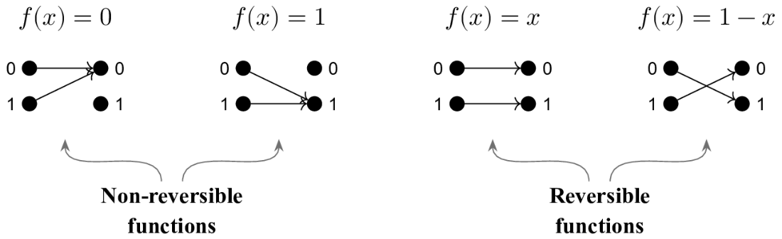
Functions \(f(x) = 0\) and \(f(x) = 1\) are non-reversible: both inputs give the same output. Functions \(f(x) = x\) and \(f(x) = 1 - x\) are reversible: different inputs are mapped to different outputs, so you can figure out which input produced the given output.
The single-bit function can be reversible, like \(f(x) = x\), or not, like \(f(x) = 1\). Adding an extra bit to the input and output allows us to define the extended function \(F(x, y)\) to be reversible regardless of whether the original single-bit function was reversible.
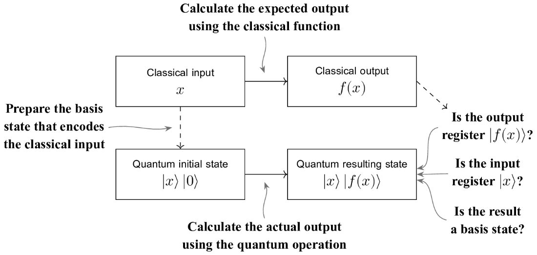
To test reversible calculations, we verify that the quantum operation produces the expected results on all basis states. For each input \(x\), we prepare the quantum input in the state \(\ket{x}\) and the output in the \(\ket{0}\) state and apply the quantum operation. The test then runs a series of checks on the resulting state, using the classically computed value \(f(x)\) as part of the verification process.
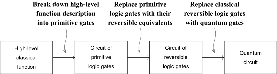
To convert a classical function into its quantum implementation, we start by representing it as a sequence of Boolean logic gates. Then, we replace each gate with its classical reversible equivalent. Finally, each classical reversible logic gate is replaced with a quantum gate that implements it.
Summary
- Solving a classical problem on a quantum computer starts with converting the classical problem description to a “quantum” formulation, which then is used to implement the quantum algorithm for solving this problem. This is called reversible computing.
- When converting a classical function \(f(x)\) to a quantum computation, classical variables are mapped onto qubit arrays, and classical computations — onto unitary transformations. The goal is to find a sequence of quantum gates that mimics the classical function evaluation, transforming the input array in any basis state \(\ket{x}\) so that the value of \(f(x)\) is encoded in the result.
- A classical function is reversible if it converts each input to exactly one output, and each output is produced by exactly one input.
- The systematic approach to implementing a classical function as a quantum computation starts with writing the process of its evaluation as a sequence of primitive logic gates. Each logic gate is then replaced by its reversible equivalent, and finally, these are replaced with their quantum gate implementations.
- Reversible computing defines the behavior of a quantum operation by specifying its effects on all basis states based on the classical function this operation implements. Its effect on a superposition state is then defined as a linear combination of its effects on individual basis states that are part of that superposition state.
- You can make any non-reversible function reversible by extending its inputs and outputs, keeping the inputs as part of the output and using a separate output bit to calculate the function value.
- You can allocate extra qubits, called auxiliary qubits, to store the values of temporary variables during the computations.
- Uncomputation involves applying adjoint of the parts of the computation you used to get the final result. You need to uncompute any changes you have done to the states of the input qubits and the auxiliary qubits to make sure your computation doesn’t introduce any unexpected side effects.
FAQ
What does it mean to “evaluate a classical function on a quantum computer”?
It means implementing a unitary U_f that embeds the classical function f into a reversible quantum transformation. The standard pattern keeps the input intact and writes the result into a separate output register: U_f |x>|y> = |x>|y ⊕ f(x)>. Here, ⊕ is XOR (addition mod 2). This form is reversible, works on superpositions by linearity, and lets you compose computations without destroying inputs.
Why must classical computations be made reversible for quantum implementation?
Quantum gates are unitary (invertible), so any computation you run must be logically reversible. Many classical functions aren’t: they map multiple inputs to the same output (e.g., f(x)=0). To implement them as quantum circuits, you extend them so inputs can be recovered from outputs—typically by preserving inputs and writing f(x) into separate target qubits via y ⊕ f(x). Measurements are avoided because they’re irreversible and would collapse superpositions.
How do we handle non‑reversible functions like f(x)=0 or f(x)=1?
Extend the function to act on an input and a target bit: F(x,y) = (x, y ⊕ f(x)). Examples:
- f(x)=0: F(x,y)=(x,y) → do nothing.
- f(x)=1: F(x,y)=(x,y⊕1) → apply X to the target.
- f(x)=x: out‑of‑place XOR → CNOT(control=x, target=y).
- f(x)=1−x: controlled-on-zero X on the target (or X on target followed by CNOT).
What is the U_f |x>|y> → |x>|y ⊕ f(x)> pattern and why is it used?
It’s the canonical reversible embedding of a classical function. Benefits:
- Reversible by construction (inputs are preserved).
- Composes cleanly with other steps.
- Extends to superpositions: by linearity, the map applies to each basis component, so U_f ∑ a_xy|x>|y> = ∑ a_xy|x>|y ⊕ f(x)>.
How can I test a reversible quantum implementation against its classical specification?
For each basis input x:
- Prepare |x>|0> and classically compute f(x).
- Apply the quantum operation.
- Check that the output qubit(s) encode f(x) and the input qubits remain |x>.
A practical trick is to “zero out” success: flip the output by X if f(x)=1 and undo the input preparation, so a correct circuit ends in |00…0>. In simulators: Qiskit uses save_statevector; Q# can use CheckAllZero or DumpMachine. Avoid gates that introduce superposition or relative phase when testing pure reversible logic.
How are basic Boolean gates implemented as quantum circuits?
Out‑of‑place versions (inputs preserved, result in target):
- NOT: X on target after CNOT from input (or controlled‑on‑zero X). In‑place NOT is simply X.
- XOR (x₀ ⊕ x₁): two CNOTs to the target, controlled by x₀ and x₁.
- Equality (x₀ == x₁): XOR to target, then X on target (negate the XOR).
- AND: multi‑controlled X (CCNOT for two inputs) with inputs as controls, target as output.
- OR: via De Morgan: OR(x₀,x₁) = NOT(AND(NOT x₀, NOT x₁)). Efficiently, use a controlled‑on‑zero multi‑controlled X to the target, then X on the target.
What is Bennett’s trick and when do I need it?
Bennett’s trick disentangles and clears temporary (ancilla) qubits without measurement. Steps:
- Compute the function into an auxiliary output register using ancillas.
- Copy the result into the final output (e.g., by CNOTs to the output).
- Uncompute: apply the inverse of the computation to return all ancillas to |0>.
Use it whenever intermediate ancillas become entangled with inputs/outputs. This prevents unwanted entanglement from spoiling later interference or correctness.
What are auxiliary (ancilla) qubits and how should I manage them?
Ancillas are temporary qubits used to store intermediate results (e.g., clause values in a CNF). Best practices:
- Initialize ancillas to |0>, use them for intermediate steps, and return them to |0> before release.
- Uncompute any changes (often the same circuit structure reversed) to remove entanglement.
- Tooling differences: Q# lets you allocate ancillas inside operations (within-apply simplifies compute/uncompute). In Qiskit, you predefine circuit width and manage ancilla indices explicitly.
What is the “synthesis of reversible logic circuits” workflow?
A systematic path from high-level classical functions to quantum circuits:
- Logic synthesis: decompose the function into Boolean primitives (AND/OR/NOT, XOR, etc.).
- Make it reversible: preserve inputs and write outputs via y ⊕ f(x); add ancillas as needed.
- Map to quantum: replace reversible gates with quantum gates (X, CNOT, multi‑controlled X, controlled‑on‑zero variants), optimize, and add uncomputation.
How do I evaluate a Boolean expression in CNF (AND of ORs) on a quantum computer?
Given n inputs and a list of clauses (each an OR of literals):
- Allocate one ancilla per clause.
- For each clause, implement its OR into its ancilla. Handle negated literals by temporarily flipping their variables (X) or using controlled‑on‑zero controls; then uncompute those flips.
- AND all clause ancillas into the final output using a multi‑controlled X.
- Uncompute each clause ancilla to return ancillas to |0> and release them.
Are there notable practical differences between Qiskit and Q# for reversible computing?
Yes:
- Ancilla management: Q# lets you allocate ancillas locally (use clauseResults = Qubit[n]) and enforces returning them to |0>; Qiskit circuits have a fixed size, so you preallocate and track indices.
- Conjugation: Q# has within/apply to structure compute–use–uncompute. In Qiskit you manually append the forward and reverse operations.
- Controls: Both support multi‑controlled X; controlled‑on‑zero is native in many toolkits (or emulate by surrounding controls with X).

 Quantum Programming in Depth ebook for free
