7 Quantizing Large Language Models in Practice

This chapter explains why large language models require a different quantization mindset than earlier networks: their activations contain a small set of extreme outlier channels that are shared across layers, and those channels are too important to clip away. It also highlights the serving-time bottleneck created by the KV cache, which can grow to match or exceed the model’s own memory footprint during long-context generation. Together, these realities make standard uniform INT8 approaches fail and motivate methods that preserve critical dimensions while still reducing memory and improving throughput.

The chapter then develops three weight-side solutions. LLM.int8() handles outliers dynamically by routing a tiny fraction of activation dimensions through full precision while quantizing the rest, achieving FP16-level perplexity with much lower memory use and no calibration. GPTQ instead uses second-order information from the Hessian to compensate for rounding errors as weights are quantized column by column, enabling strong 4-bit and even 3-bit compression with minimal quality loss. AWQ takes a simpler preventive approach by using activation statistics to identify important channels, scaling them before quantization so that the sensitive weights land on finer grid points and standard rounding works well.

Finally, the chapter extends quantization to the KV cache with TurboQuant, which uses a random rotation and precomputed codebooks to compress vectors on arrival without calibration. It compares all methods in terms of accuracy, memory, deployment time, and robustness, showing that they are complementary rather than mutually exclusive. The practical takeaway is a deployment strategy: use LLM.int8() when speed of setup matters most, GPTQ when squeezing maximum quality from aggressive weight compression, AWQ when robustness and production serving are priorities, and TurboQuant when KV-cache memory is the limiting factor, often stacking it with a weight method for the best overall footprint.

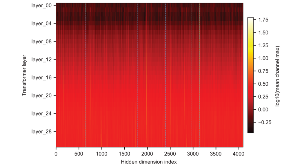
Per-channel activation magnitude heatmap for OPT-6.7B (32 layers × 4,096 hidden dimensions, log scale). Bright vertical stripes mark the same hidden dimensions spiking across all layers. Dashed lines mark the five universal outlier channels—dimensions 639, 1778, 2394, 2972, and 3136—that appear in the top 1% of every layer.

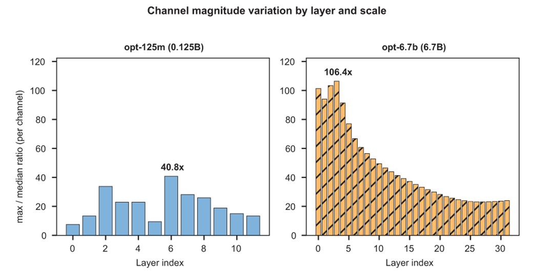
Channel magnitude variation across model scales. Left: OPT-125M shows sporadic spikes with no consistent pattern across layers. Right: OPT-6.7B shows sustained high ratios (max/median above 23× everywhere, 106× peak) that decrease smoothly from early to late layers. Shared Y-axis makes the severity contrast visible. Numbers above bars indicate the peak ratio per model.

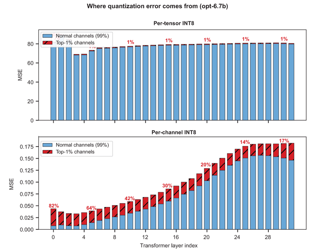
Where quantization error comes from in OPT-6.7B. Top: under per-tensor INT8, the top-1% channels (40 of 4,096) contribute only ~1% of MSE—they set the scale and quantize cleanly. The 99% of normal channels absorb the error. Bottom: per-channel INT8 reduces total MSE by 1,872× (layer 0) to 442× (layer 31), but outlier dims still account for 82% of residual error in early layers—motivating decomposition into separate precision paths.

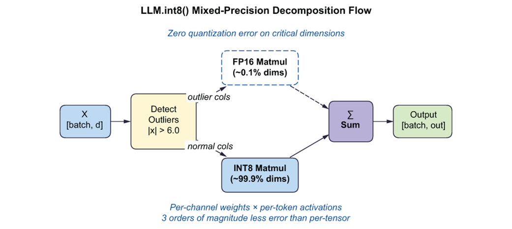
LLM.int8() mixed-precision decomposition flow. Input activations are scanned for outlier dimensions (|x| > 6.0). The ~0.1% of dimensions that exceed the threshold are routed to a full-precision matmul (dashed path); the remaining ~99.9% are quantized to INT8. Summing the two outputs recovers the full result with zero quantization error on the critical dimensions and per-channel × per-token precision on everything else.

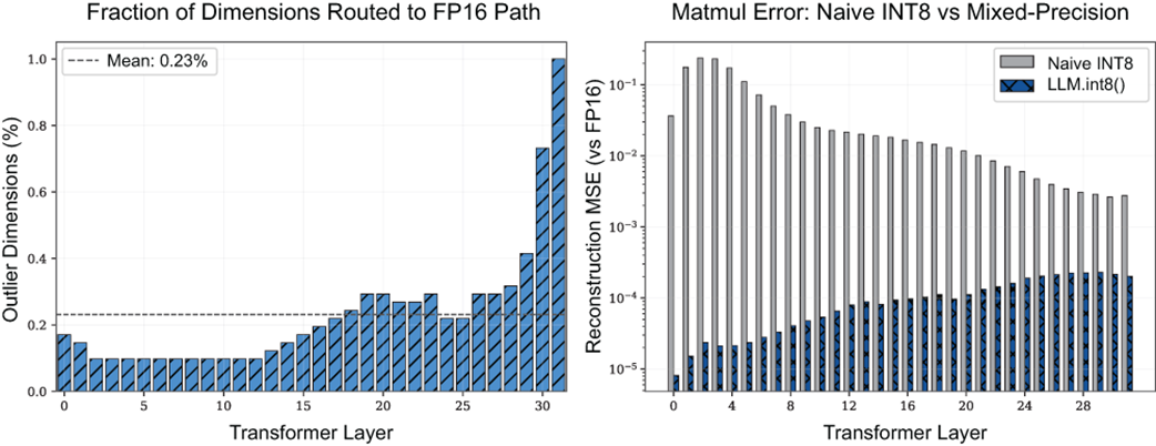
Decomposition anatomy for OPT-6.7B. Left: fraction of dimensions routed to the FP16 path per layer (mean 0.23%, dashed line). The overhead increases from ~0.1% in early layers to 1.0% in the last layer, but stays below 1% everywhere except layer 31. Right: reconstruction MSE vs FP16 on a log scale. Filled bars show naive INT8 error; hatched bars show the mixed-precision error. The gap ranges from 4 orders of magnitude in early layers to just over 1 order in late layers.

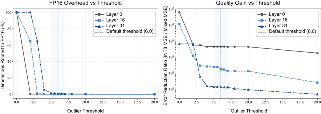
Threshold sweep for OPT-6.7B. Left: fraction of dimensions routed to FP16 as a function of threshold. Right: error reduction ratio (log scale). The shaded band marks the 5.0-7.0 sweet spot. Each layer reveals a different personality: layer 0 (circles, solid) is threshold-insensitive, layer 16 (squares, dashed) shows the clearest knee at 6.0, and layer 31 (triangles, dash-dot) has broadly elevated activations requiring more outlier routing at any threshold.

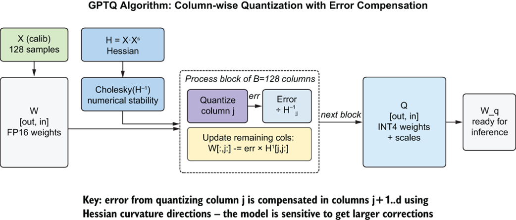
GPTQ algorithm flow. Calibration activations X produce the Hessian H = XXT, which is Cholesky-factored for numerical stability. The weight matrix W is processed in blocks of B=128 columns. Within each block, each column is quantized to INT4, and the rounding error is distributed across remaining columns using the inverse Hessian. The output is the quantized weight matrix Q plus per-group scales.

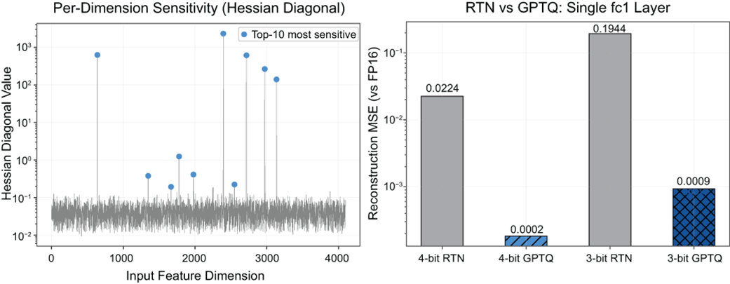
Left: Hessian diagonal for OPT-6.7B layer 0 fc1. Most of the 4,096 input dimensions have low sensitivity (baseline ~0.04), but the top-10 dimensions spike to 100–1,000×, matching the outlier channels from Section 7.1. Right: reconstruction MSE for RTN vs GPTQ on this single layer. At 4-bit, GPTQ reduces error by 112× (0.0224 → 0.0002). At 3-bit, the advantage grows to 216× (0.1944 → 0.0009)—Hessian-aware error compensation becomes more valuable as the grid gets coarser.

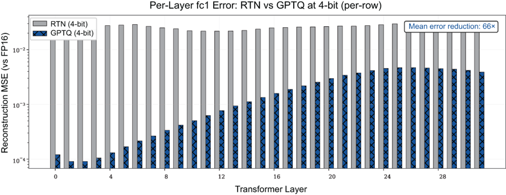
Per-layer fc1 reconstruction MSE for RTN vs GPTQ (cross-hatched) at 4-bit per-row quantization across all 32 transformer layers in OPT-6.7B. GPTQ reduces error in every layer, with a mean improvement of 66×. Both methods show increasing MSE in later layers, but GPTQ's advantage holds throughout.

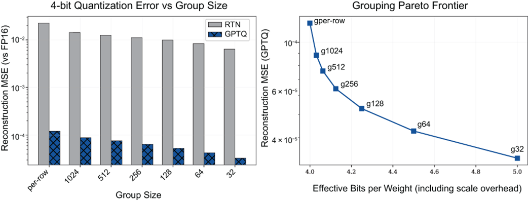
Left: reconstruction MSE at different group sizes for RTN and GPTQ (cross-hatched). Both methods improve with smaller groups, but GPTQ improves faster—its advantage over RTN grows as groups get finer. Right: GPTQ's Pareto frontier of reconstruction MSE vs effective bits per weight (including the FP16 scale and zero-point overhead per group). Group size 128 sits at the knee—further shrinking to 64 or 32 yields diminishing MSE returns at increasing storage cost.

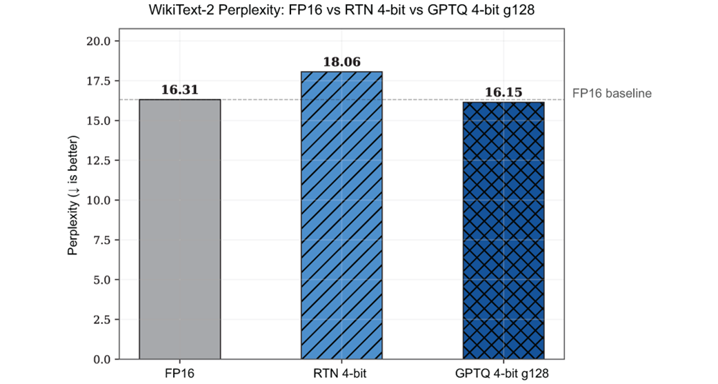
WikiText-2 perplexity for OPT-6.7B. FP16 baseline (16.31) compared to RTN 4-bit per-row (hatched, 18.06) and GPTQ 4-bit g128 (cross-hatched, 16.15). The dashed line marks the FP16 baseline. RTN degrades perplexity by 10.7%. GPTQ avoids degradation entirely—scoring 0.16 points below FP16 (within measurement noise at this evaluation length) while loading in 3,626 MB vs FP16's 12,700 MB.

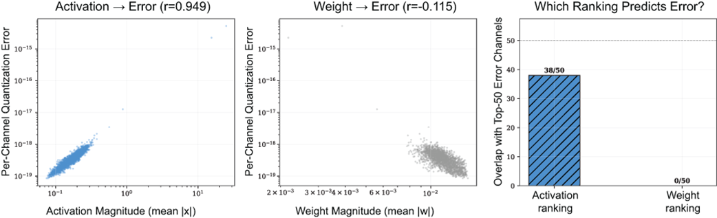
Which ranking predicts quantization error? Left: activation magnitude vs per-channel quantization error (r = 0.949, strong positive correlation). Center: weight magnitude vs the same error (r = −0.115, no useful correlation). Right: of the 50 channels with the highest true quantization error, activation ranking identifies 38 of them; weight ranking identifies zero. Activation magnitude is the correct importance signal for weight quantization.

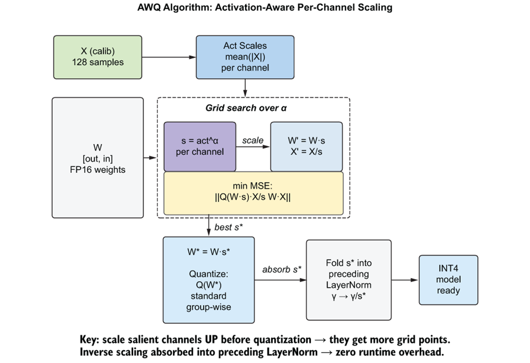
AWQ algorithm flow. Calibration data produces per-channel activation scales (top). A grid search over the scaling exponent α finds the best per-channel scale vector s* that minimizes reconstruction error after quantization (center). The optimal scales are applied to weights before standard group-wise quantization, then the inverse is folded into the preceding LayerNorm—producing an INT4 model with zero runtime overhead.

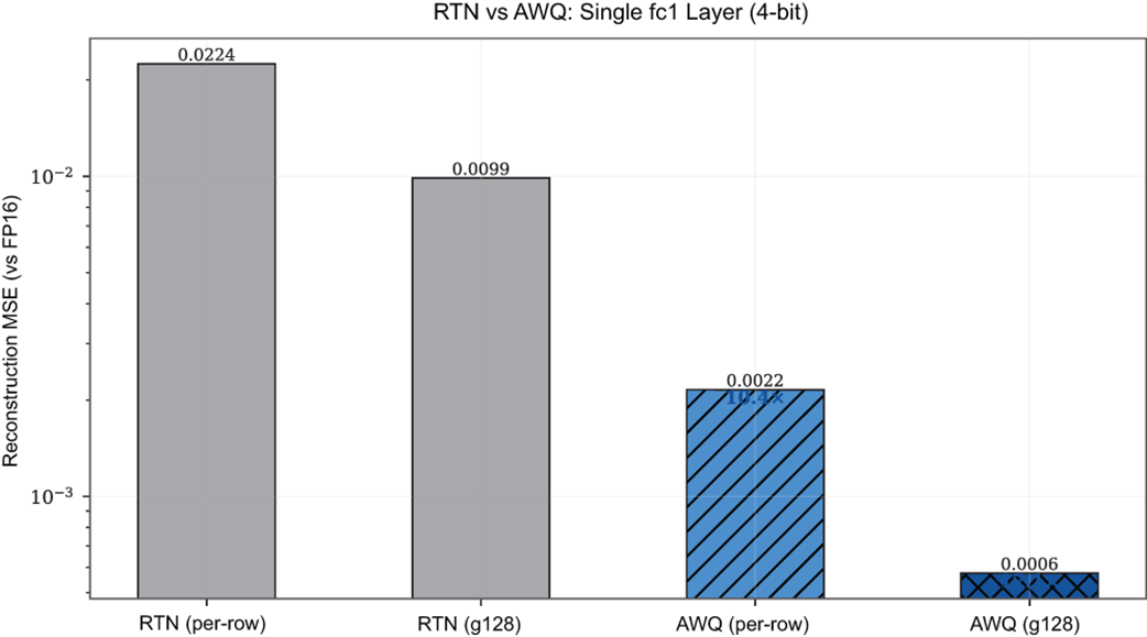
Reconstruction MSE on a single fc1 layer (OPT-6.7B, layer 0, 4-bit). AWQ reduces error by 10.4× with per-row quantization and 17.1× with group size 128. The combination of AWQ scaling and group quantization is multiplicative: group-128 gives RTN a 2.3× boost (0.0224 → 0.0099), but gives AWQ a 3.8× boost (0.0022 → 0.0006) because finer groups interact constructively with per-channel scaling.

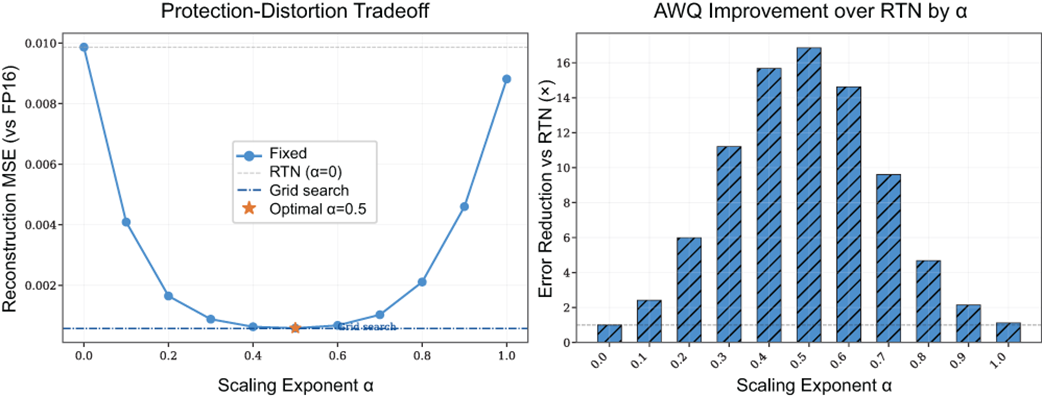
The protection-distortion tradeoff. Left: reconstruction MSE as a function of the scaling exponent α. The curve is U-shaped—too little scaling (α near 0) leaves salient channels unprotected; too much (α near 1) inflates the group scale for non-salient channels. The optimal α = 0.5 achieves 16.9× error reduction versus RTN, nearly matching the full grid search (17.1×, dashed line). Right: error reduction ratio versus RTN at each α. The sweet spot is broad—any α between 0.3 and 0.7 achieves at least 4.7× improvement.

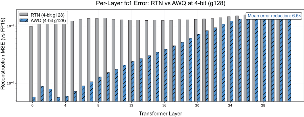
Per-layer fc1 reconstruction MSE for RTN vs AWQ (hatched) at 4-bit group-128 across all 32 transformer layers in OPT-6.7B. AWQ reduces error in every layer, with a mean improvement of 6.5×. The advantage is largest in early layers (17–21×) and diminishes in later layers (1.1×), mirroring the activation outlier concentration from Section 7.1.

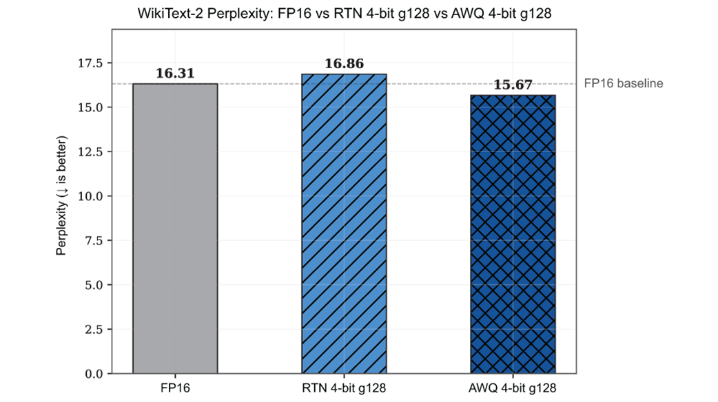
WikiText-2 perplexity for OPT-6.7B. FP16 baseline (16.31) compared to RTN 4-bit g128 (hatched, 16.86, +0.54) and AWQ 4-bit g128 (cross-hatched, 15.67, −0.64). AWQ not only eliminates the RTN degradation but scores 0.64 points below the FP16 baseline—within evaluation variance but directionally better. The AWQ model loads in 3,613 MB versus FP16's 12,700 MB.

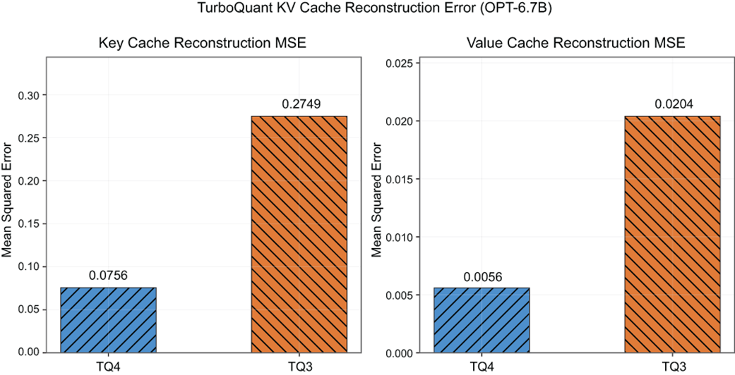
TurboQuant reconstruction MSE on OPT-6.7B KV cache (32 layers, 8 sequences). Left: key cache. Right: value cache. TQ4 key MSE is 0.0756, value MSE is 0.0056. TQ3 roughly triples both. Values reconstruct an order of magnitude more accurately than keys, mirroring the outlier channel asymmetry from Section 3.4.

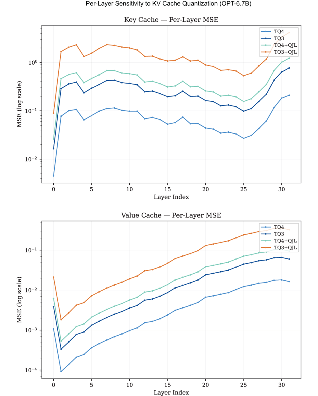
Per-layer reconstruction MSE on OPT-6.7B with and without QJL correction. MSE-only (solid lines) beats QJL-corrected (dashed lines) across all 32 layers, both bit-widths, and both keys and values. QJL TQ4 is worse than MSE-only TQ3 in most key cache layers. Log-scale Y-axis.

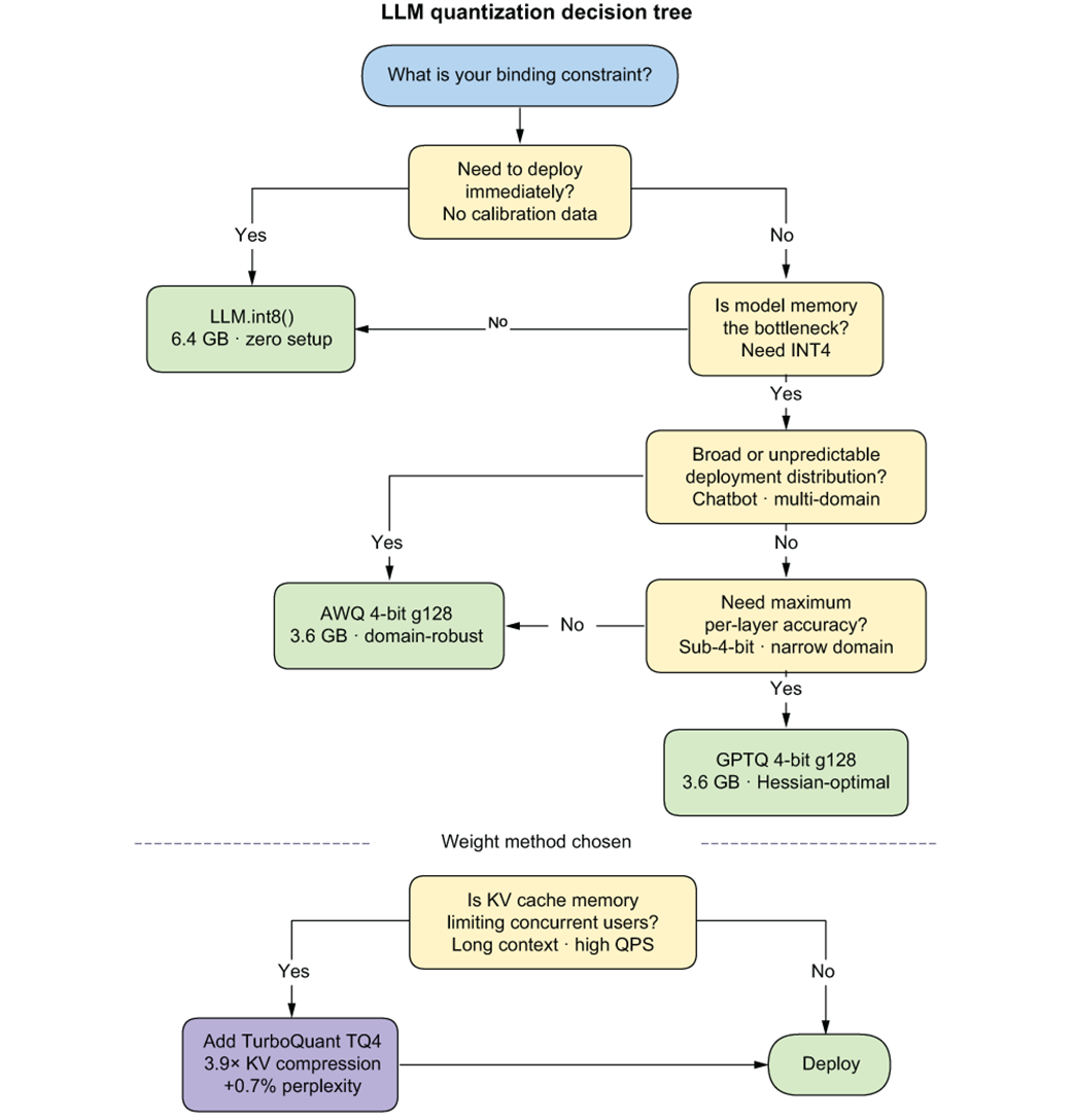
LLM quantization decision framework. Start from the binding deployment constraint and follow the branches. Weight methods (top) and KV cache methods (bottom) are orthogonal - combine them for maximum compression.

• LLM quantization is a distinct problem from the toolkit in Chapters 3–6 because activation outliers at the 7B+ scale reach 100×+ the channel median, concentrate in a handful of coordinated dimensions across all layers, and cannot be clipped without collapsing perplexity.
• LLM.int8() splits each matmul into a dense INT8 path and a tiny FP16 path for the outlier dimensions, matching FP16 quality at half the memory with no calibration data — the fastest route from model to quantized deployment.
• GPTQ quantizes weight columns left-to-right and uses the input Hessian to redistribute each column's rounding error across the remaining columns, enabling 4-bit weights with no measurable quality loss on a matched calibration distribution.
• AWQ protects the ~1% of weight channels tied to high-magnitude activations by rescaling them before round-to-nearest, trading a small amount of GPTQ's optimality for much better robustness under domain shift.
• TurboQuant compresses the KV cache online with a random rotation and a fixed codebook — no calibration — and composes with any weight method, which is how you serve long-context workloads at real concurrency.

FAQ