5 Recovering Accuracy with Quantization-Aware Training

This chapter explains when and how quantization-aware training becomes the right tool for recovering accuracy after post-training quantization is no longer enough. It starts from the idea that PTQ is usually the fastest path to INT8 deployment, but that INT4, small models, and very tight accuracy budgets can expose failures that PTQ cannot repair on its own. The core response is to train models as if quantization will happen at inference time, so they can adapt their weights to the integer grid instead of merely enduring quantization noise.

The chapter then develops the mechanics of QAT: fake quantization simulates quantized forward passes while keeping gradients usable, and the straight-through estimator supplies those gradients by treating rounding as approximately identity during backpropagation. It shows how this enables weights to migrate toward grid points, how clipped STE prevents wasted updates on saturated values, and how practical QAT implementations rely on observer modules, batch-norm folding, careful learning-rate schedules, and stability safeguards. It also emphasizes that QAT should be scheduled efficiently, with warmup, observer freezing, and progressive bit-width reduction used to minimize training cost while maintaining convergence.

Beyond the basic training loop, the chapter argues that success depends on choosing the right granularity and scope for quantization. Per-channel weight quantization usually preserves more gradient signal than per-tensor quantization, especially for convolutional and linear layers with uneven channel magnitudes, though the gain depends on model scale and structure. For transformers, the chapter recommends diagnosing sublayer sensitivity before training, then protecting the most fragile components—often the feed-forward blocks or sometimes mixed-precision holdouts—while keeping LayerNorm, softmax, and GELU in full precision. Overall, the message is to match the intervention to the failure mode: use calibration or mixed precision when that is enough, and reserve QAT for cases where diffuse or severe quantization damage truly requires retraining.

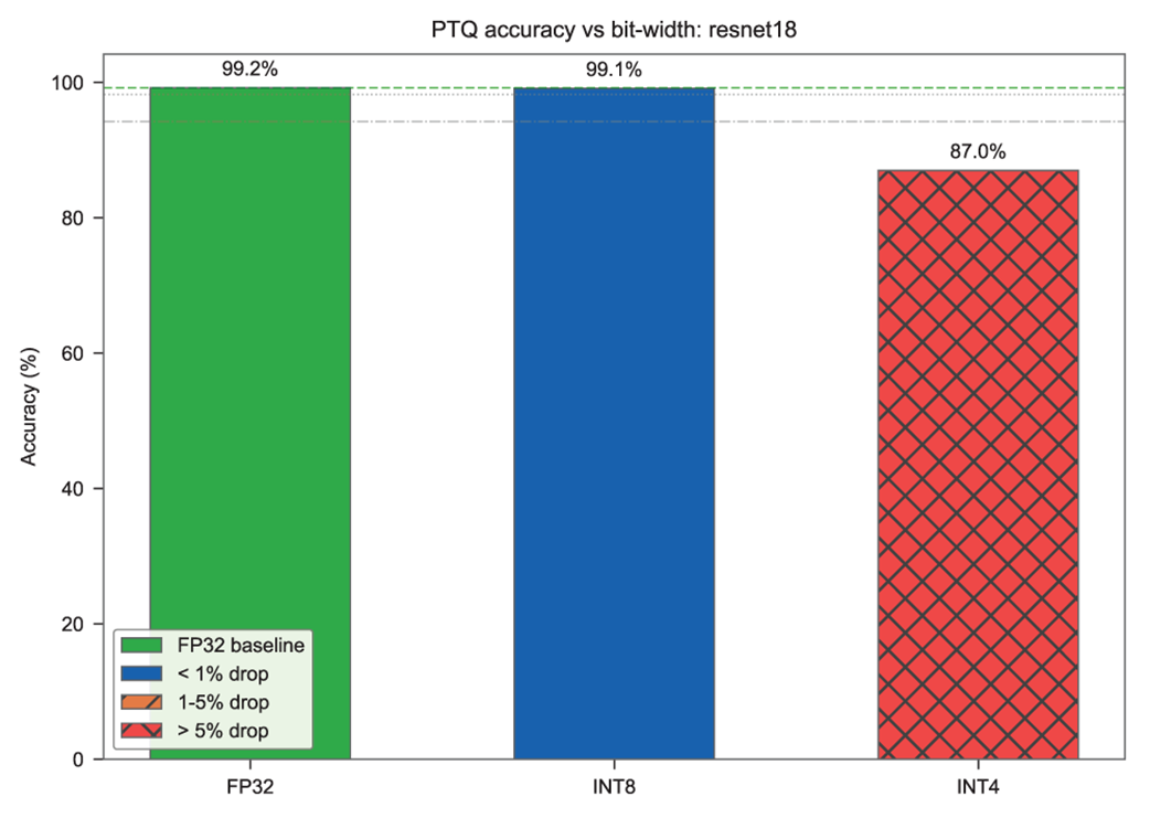
PTQ accuracy for ResNet-18 on ImageNette. INT8 is indistinguishable from the FP32 baseline. INT4 drops 12 percentage points—the model is degraded but still functioning.

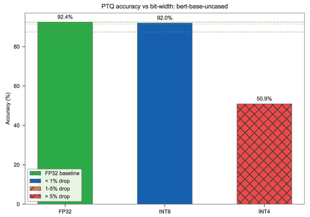
PTQ accuracy for BERT-base on SST-2. INT8 holds with under 0.5% loss. INT4 drops to 50.9%—coin-flip accuracy on a binary task, meaning the model has effectively stopped functioning.

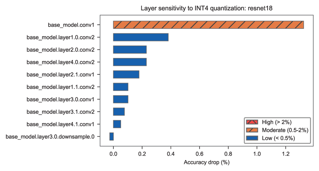
Layer sensitivity analysis for ResNet-18 at INT4. The first convolutional layer (conv1) shows the highest sensitivity at 1.32%, followed by a smooth gradient across the remaining layers. All bars are moderate or low—no single layer dominates the 12% total degradation.

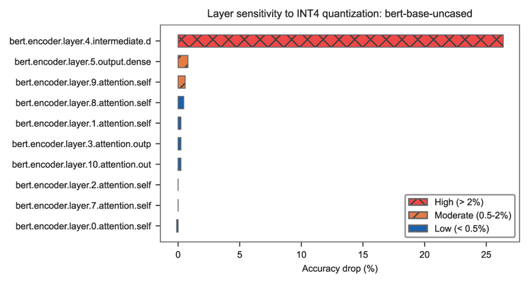
Layer sensitivity analysis for BERT at INT4. One layer dominates everything: layer.4.intermediate.dense causes a 26.4% accuracy drop when quantized alone. The remaining layers are noise in comparison. This is a concentrated failure—a clear target for mixed precision.

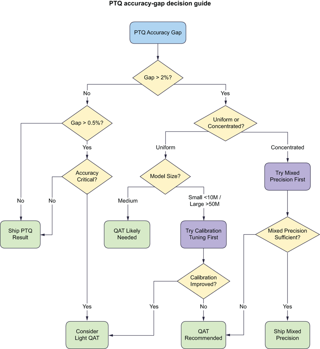
QAT decision framework. The key branch is whether failure is concentrated or diffuse—this determines whether mixed precision can save you from the cost of QAT.

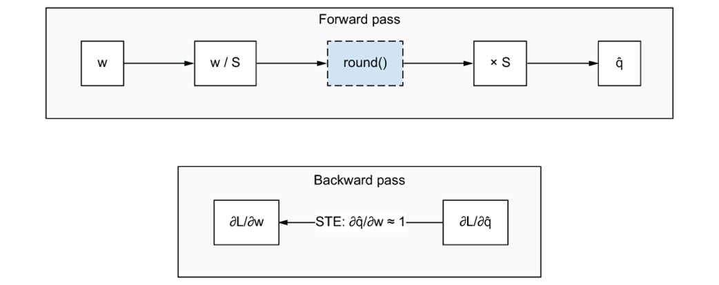
The straight-through estimator passes gradients unchanged through the non-differentiable rounding operation

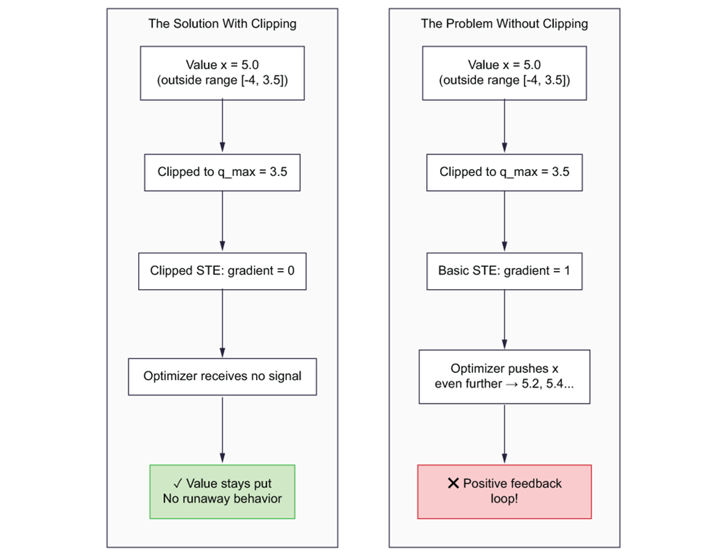
Why clipped STE zeros gradients for out-of-range values. A value clipped to the boundary is already saturated—pushing it further cannot change the quantized output. Zeroing the gradient prevents the optimizer from wasting updates on values stuck at the rails, focusing learning capacity on weights that can still move between grid points.

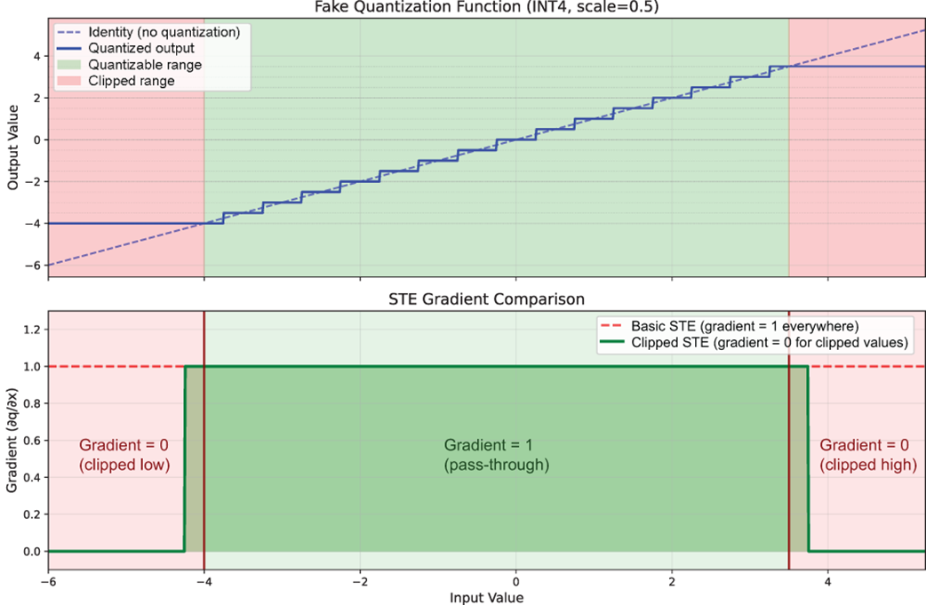
Visualizing the clipped STE gradient function. Top: the fake quantization staircase with "quantizable range" and "clipped range." Bottom: gradient behavior - basic STE (dashed) passes gradient 1 everywhere; clipped STE zeros gradients in the clipped regions.

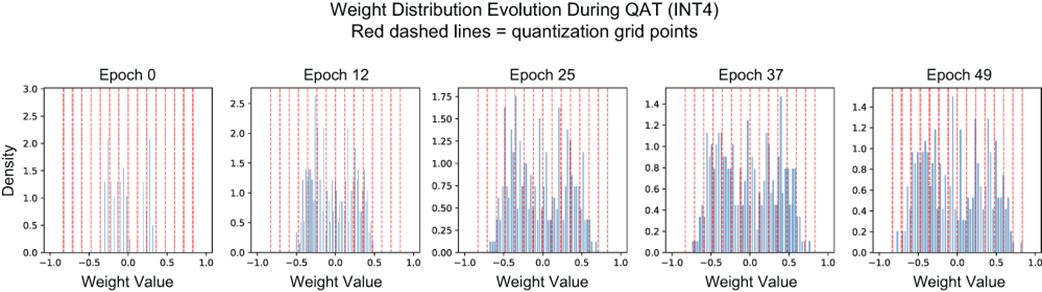
Weight distributions migrate toward INT4 grid points during QAT. Five snapshots of conv1 weights (epochs 0–49) show the initially Gaussian distribution reorganizing into sharp spikes aligned with quantization levels (dashed lines), demonstrating that QAT actively adapts weights to minimize rounding error rather than passively tolerating it.

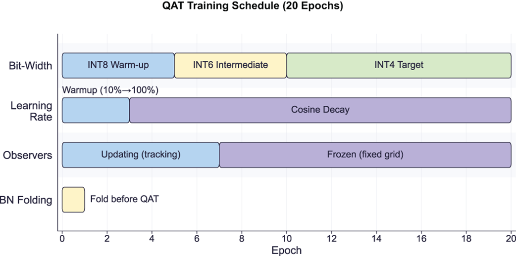
The complete QAT schedule coordinates four components. Bit-width decreases progressively (INT8→INT6→INT4). The learning rate warms up during INT8 calibration, then cosine-decays through the remaining phases. Observers freeze at epoch 8, after they've seen the INT6 distribution. Batch normalization is folded before training begins.

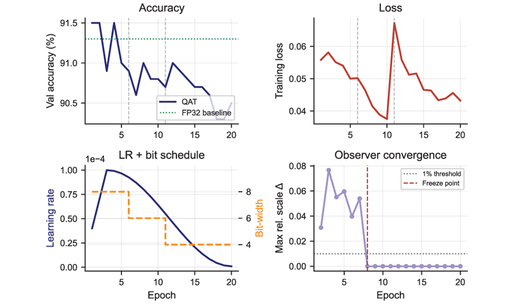
The four-panel view of the scheduled QAT pipeline. Top left: validation accuracy oscillates but stays within ~1 point of FP32 despite dropping to INT4. Top right: training loss spikes at each bit-width transition (dashed verticals at epochs 6 and 11), then recovers. Bottom left: the learning rate (solid) warms up and cosine-decays while bit-width (dashed steps) progresses 8→6→4. Bottom right: observer ΔScale spikes at bit-width transitions, then drops to zero after freezing at epoch 8.

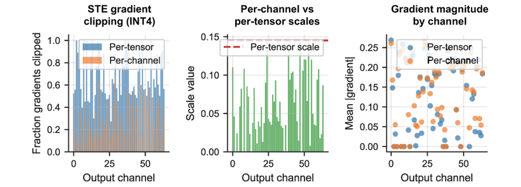
Three views of the gradient survival problem on ResNet-18 conv1 at INT4. Left: fraction of gradients clipped per output channel—per-tensor clips 100% of gradients in several channels, while per-channel stays well below 20%. Center: per-channel scales vs the single per-tensor scale —many channels have scales an order of magnitude smaller than the global maximum. Right: per-channel quantization produces more uniform gradient magnitudes across channels, while per-tensor leaves some channels with zero gradient signal.

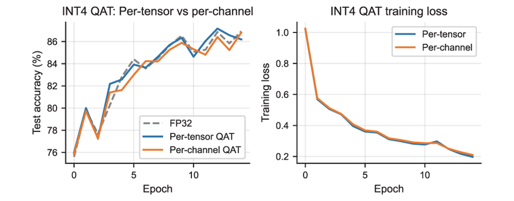
Left: Test accuracy curves for FP32, per-tensor INT4 QAT, and per-channel INT4 QAT. All three converge to nearly the same accuracy (~87%). Right: Training loss curves are virtually indistinguishable between the two QAT strategies.

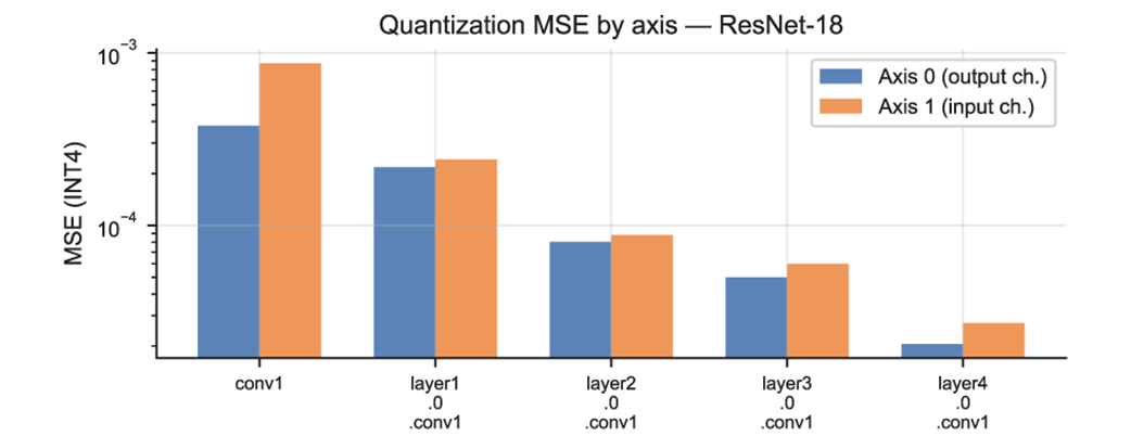
INT4 quantization MSE by axis for five ResNet-18 convolutional layers. Axis 0 produces lower MSE than axis 1 in every layer. The advantage is most pronounced in conv1, where the asymmetry between 64 output and 3 input channels is extreme.

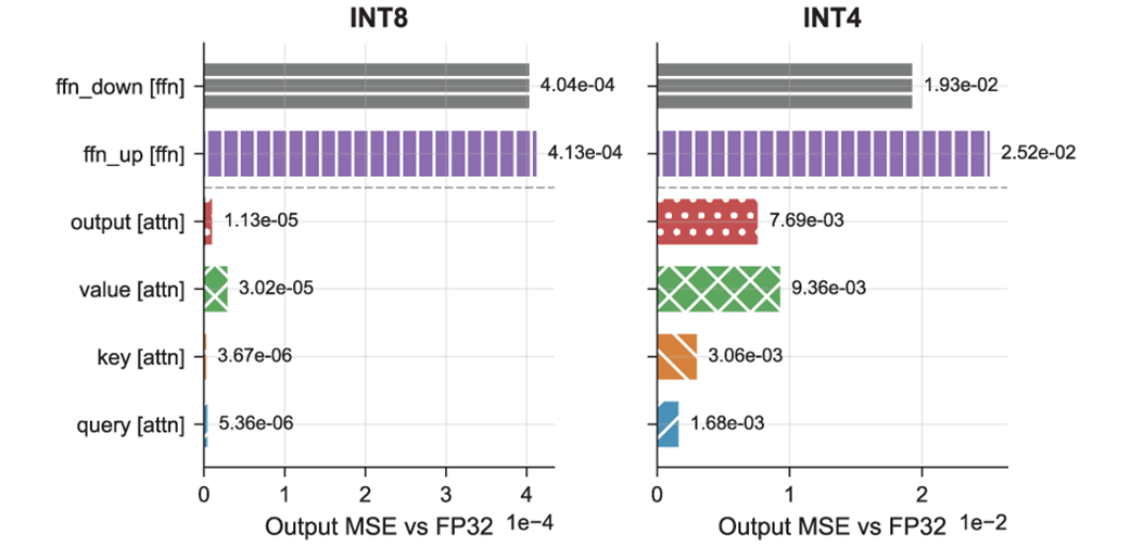
Sublayer sensitivity to per-channel weight fake quantization on BERT-base-uncased. FFN sublayers dominate—16.2× more aggregate output MSE than all four attention projections at INT8, 2.0× at INT4. Dashed line separates attention (below) from FFN (above).

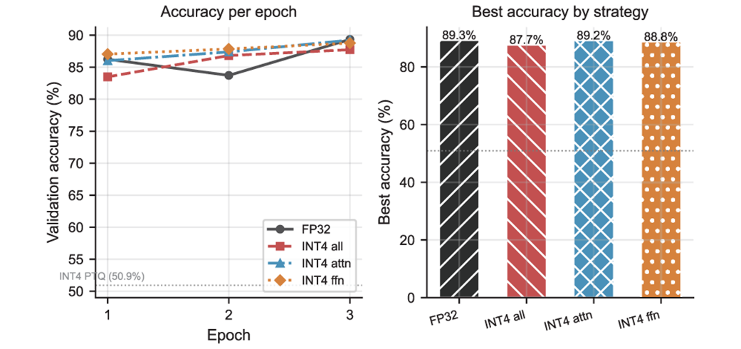
Selective QAT fine-tuning on SST-2 (INT4, 3 epochs). Left: accuracy per epoch. Right: best accuracy by strategy. QAT recovers BERT from the INT4 PTQ catastrophe (50.9%) to within 1.6% of FP32. Attention-only (48 layers at INT4) nearly matches FP32 at just −0.11%. FFN-only (24 layers) costs −0.57%. Quantizing all 72 layers incurs the largest gap (−1.61%).

• QAT is warranted when PTQ fails at your target bit-width, but the failure pattern determines the intervention. INT4 PTQ dropped ResNet-18 by 12 percentage points (diffuse, across all layers) and collapsed BERT-base to 50.9% coin-flip accuracy (concentrated in a single FFN layer). Diffuse failure needs QAT; concentrated failure needs mixed precision. Always run layer sensitivity before choosing.
• Fake quantization inserts quantize-then-dequantize operations into the forward pass so the model trains against quantization noise while gradients flow through the straight-through estimator. The clipped STE—which zeros gradients for out-of-range values—is the recommended default. Use lower learning rates (1e-4 to 1e-5), shorter schedules (5–20 epochs), and gradient clipping.
• Scheduling reduces QAT cost without sacrificing accuracy. Warm up the learning rate for 10–15% of total epochs, freeze observers once per-layer scale changes drop below 1%, and progress bit-width gradually (INT8→INT6→INT4). Our scheduled pipeline reached 90.30% on SmallCNN at INT4—slightly above the FP32 baseline—with the same wall-clock time as naïve QAT.
• Per-channel fake quantization prevents gradient starvation during QAT. Per-tensor INT4 quantization clips 100% of gradients in some output channels; per-channel keeps all channels below 20%. Quantize along axis 0 (output channels) for both convolutions and linear layers.
• Transformer QAT requires selective application. FFN sublayers produce 16.2× more aggregate output MSE than attention projections at INT8. Attention-only QAT recovered BERT from 50.9% to within 0.11% of FP32; quantizing all layers incurred 1.61%. Always keep LayerNorm, softmax, and GELU in FP32—their parameter count is negligible but their numerical sensitivity is high.
• When diminishing returns set in, stop. Monitor observer ΔScale and validation accuracy jointly—when per-layer scale changes flatten below 1% and accuracy stops recovering after bit-width transitions, further epochs add cost without benefit.

FAQ