2 Building Quantization from First Principles
This chapter explains quantization as the bridge between floating-point training and integer-based inference hardware. It begins with fixed-point numbers, showing how hardware stores integers that are interpreted through an imaginary binary point, and uses simple examples to make two’s complement, wraparound behavior, and saturation intuitive. From there, it motivates why deep learning needs more flexibility than rigid fixed-point rules can provide, especially when tensors vary widely in scale and shape.
The core mathematical development is the affine quantization map, which introduces a scale and zero-point so each tensor can use a custom integer grid. The scale sets the step size or resolution, while the zero-point shifts the grid so real zero is exactly representable, which is crucial for padding and sparsity. The chapter also derives how these parameters are chosen from data ranges, shows how quantization and dequantization work in practice, and compares per-tensor, per-channel, and group-wise granularity choices as different ways to balance accuracy against implementation cost.
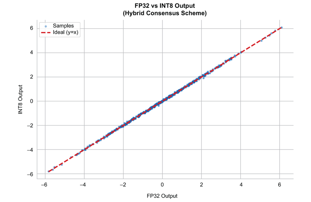
The chapter then analyzes the two main sources of error: granular error from rounding values that fall between grid points, and overload error from clipping values outside the representable range. These errors trade off against one another, so calibration is really about choosing where distortion should occur. Finally, it compares symmetric and asymmetric schemes, arguing for a hybrid approach in which weights are usually symmetric for efficiency while activations are often asymmetric for better use of the available codes. End-to-end PyTorch examples confirm that this combination can closely match full-precision results, while also showing how zero-point correction becomes essential when activations are shifted away from zero.
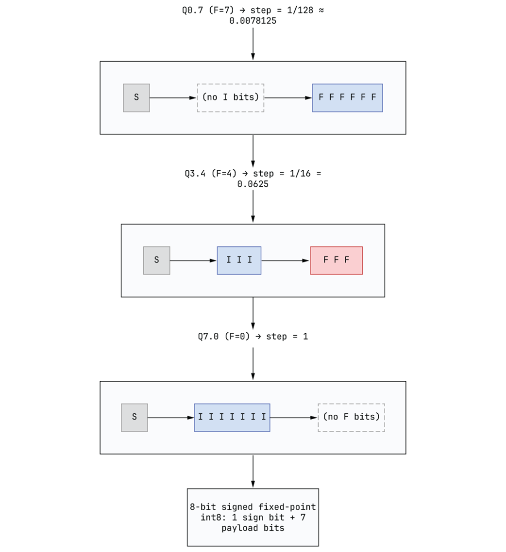
The Q3.4 fixed-point format divides 8 bits into a sign bit, 3 integer bits, and 4 fractional bits. Here, the bit pattern 0 001 1000 encodes +1.5 — the integer bits 001 contribute 1, and the leading fractional bit 1000 contributes 2-¹ = 0.5.

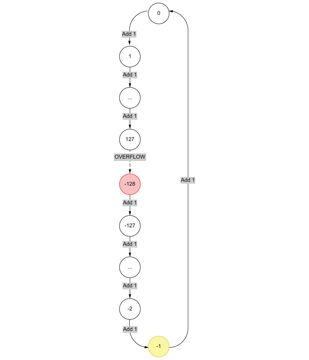
The 8-bit signed integer ring. The 256 possible bit patterns wrap around a circle, with 0 at the top and −1 (1111 1111) one step below it. Moving clockwise increments the integer; moving counterclockwise decrements it.
The range-versus-precision tradeoff in Q-format. For a fixed 8-bit container, every bit allocated to the integer part doubles the representable range but halves the precision (step size). Moving the binary point left (more fractional bits) gives finer resolution at the cost of a narrower range; moving it right does the reverse. There is no free lunch: the total information capacity is fixed by the bit-width.
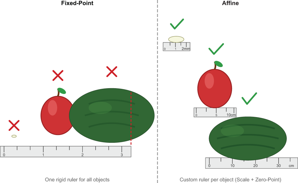
The ruler problem. Fixed-point quantization (left) forces a single rigid ruler on all measurements: a rice grain vanishes between coarse tick marks, while a watermelon extends beyond the ruler's edge and gets clipped. Affine quantization (right) manufactures a custom ruler for each object, with tick spacing (scale) and starting position (zero-point) tailored to the data's actual range.
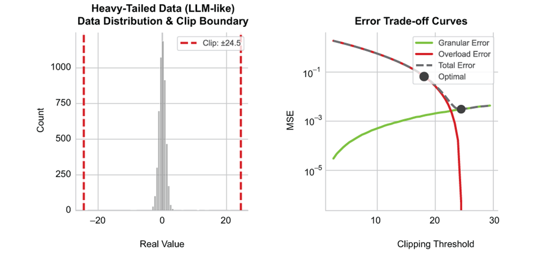
The granular-versus-overload error tradeoff. Widening the quantization grid (increasing the clipping range) reduces overload error—fewer values are clipped—but coarsens the step size, increasing granular error for values inside the range. Tightening the grid does the reverse. The optimal clipping boundary minimizes total distortion and depends on the shape of the data distribution: heavy-tailed distributions push the boundary outward; tightly concentrated distributions pull it inward.
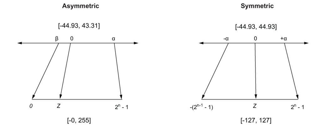
Symmetric versus asymmetric quantization. Asymmetric quantization (left) shifts the grid to cover only the region the data actually occupies, reclaiming bits that would otherwise encode empty space. The zero-point Z records the shift, and must be accounted for during inference arithmetic. Symmetric quantization (right) pins the grid at zero and mirrors the range, making it ideal for centered distributions like weight tensors but wasteful for one-sided data.
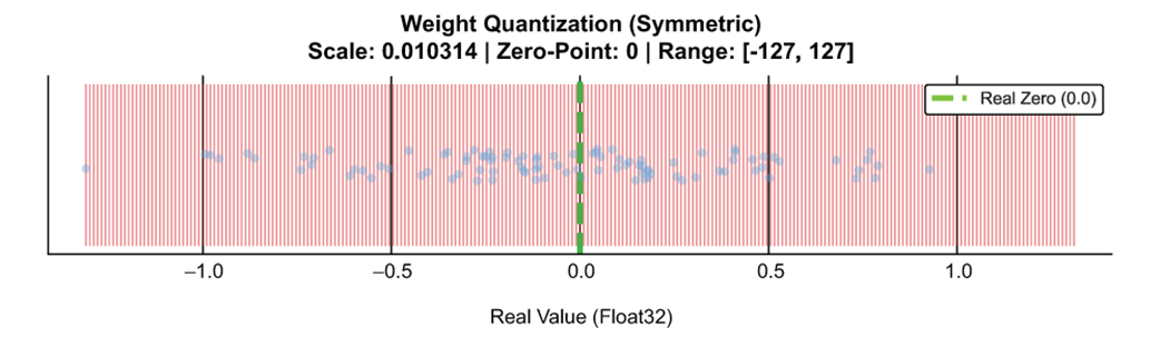
Weight quantization (symmetric)
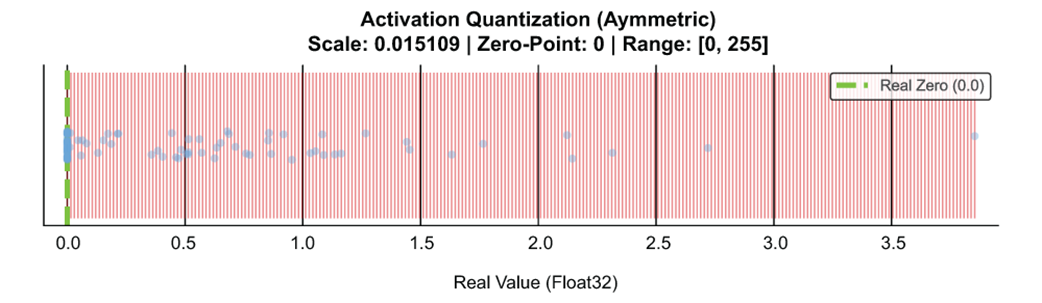
Activation quantization (affine/asymmetric)
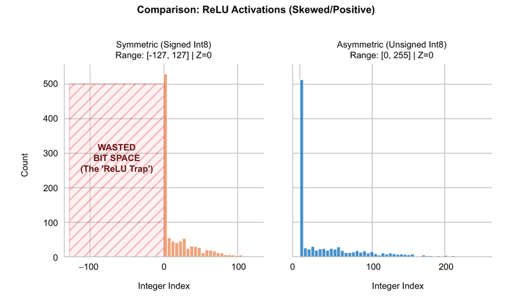
Symmetric vs asymmetric on ReLU activations
FP32 baseline vs INT8 output
Summary
- Fixed-point arithmetic stores numbers on a rigid discrete grid determined at design time. The Q-format notation makes explicit the fundamental bargain: allocate bits to range or to precision, but never both. Two's complement representation enables negative numbers through overflow, while saturation at the overflow cliff constrains every fixed-point system.
- The affine transformation r = S(q - Z) bridges floating-point tensors and integer storage. Scale (S) is the ratio of real range to integer range; zero-point (Z) aligns real zero with an integer coordinate. The zero-point nudge forces the calibrated range to include 0.0, preserving sparsity after ReLU and enabling correct zero-padding.
- Granular error arises when values land between grid points and must be rounded, bounded by S/2. Overload error arises when values fall outside the grid and are clipped, introducing unbounded distortion. Widening the grid reduces clipping but increases rounding; tightening it does the reverse.
- Symmetric quantization centers the grid on zero, wasting capacity on one-sided distributions but eliminating cross-term overhead. Asymmetric quantization shifts the grid to follow data, reclaiming bits at the cost of runtime correction. The Hybrid Consensus—symmetric weights, asymmetric activations—matches each scheme to its statistical reality.
- Visualization reveals wasted bits immediately: if half the integer codes cover empty space, the wrong scheme was chosen. The quantized arithmetic, when implemented correctly with zero-point correction, matches FP32 output to within the noise floor of 8-bit representation.
- Calibration is not a one-time event. Scale and zero-point derivations in this chapter assumed known min/max—true for weights but not activations, whose ranges shift with every batch. Strategies like percentile clipping and entropy minimization replace raw min/max with robust boundaries; when input distributions drift, recalibration may be needed.

 Quantization and Fast Inference ebook for free