This chapter introduces unsupervised methods as tools for discovering latent structure in data when no target outcome is specified. Rather than predicting, the goal is to reveal patterns that can guide understanding, feature engineering, and subsequent supervised modeling. The focus is on two complementary techniques: cluster analysis, which groups similar observations, and association rule mining, which uncovers items or attributes that frequently co-occur. Throughout, the chapter emphasizes that unsupervised work is exploratory and iterative, demanding careful choices of distance metrics, data scaling, and validation criteria to separate meaningful structure from artifacts.
The clustering portion covers how to define similarity and distance (Euclidean, Manhattan, Hamming, cosine), why units and scaling matter, and how to apply hierarchical clustering and k-means in practice. It demonstrates building distance matrices, using Ward’s method, and visualizing results via projections onto principal components. Methods for selecting the number of clusters include inspecting the elbow in total within sum of squares, the Calinski–Harabasz index, and silhouette width, with the gap statistic noted as another option. Cluster stability is assessed through bootstrap resampling with the Jaccard coefficient, helping flag “miscellaneous” clusters that do not persist. Practical guidance includes assigning new points to the nearest centroid of discovered clusters and remembering that different algorithms, metrics, and scalings can yield different yet defensible partitions.
The association rules section reframes the data as transactions and items, then mines rules of the form “if X then Y” using the apriori algorithm. Core measures include support (prevalence), confidence (rule accuracy), and lift (departure from chance co-occurrence), with additional diagnostics such as coverage (how often a rule can be applied) and Fisher’s exact test (significance). The workflow illustrates reading sparse transaction data, exploring basket sizes and item frequencies, setting appropriately low support thresholds in high-dimensional settings, and interactively sifting many rules by sorting, filtering, and constraining which items may appear on the left or right side of a rule. The result is a practical recipe for turning raw co-occurrence data into actionable recommendations and merchandising insights while remaining vigilant about rarity, spurious patterns, and domain relevance.
Figure 9.1. Mental Model
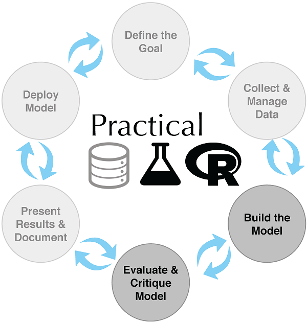
Figure 9.2. An example of data in three clusters
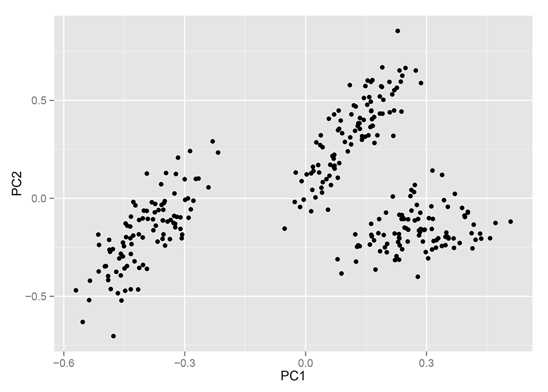
Figure 9.3. Manhattan versus Euclidean distance
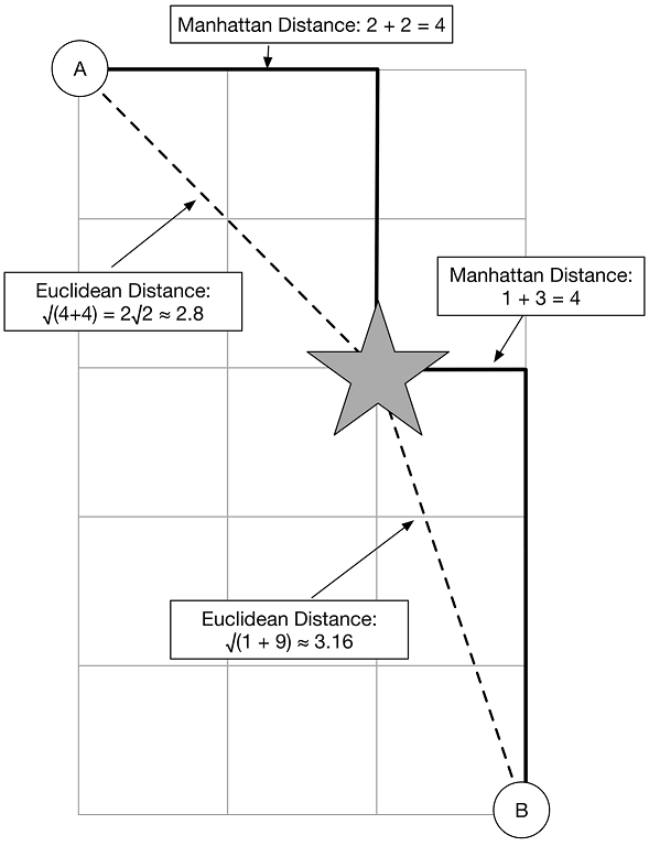
Figure 9.4. Cosine similarity
Figure 9.5. Comparison of Fr.Veg and RedMeat variables, unscaled (top) and scaled (bottom)
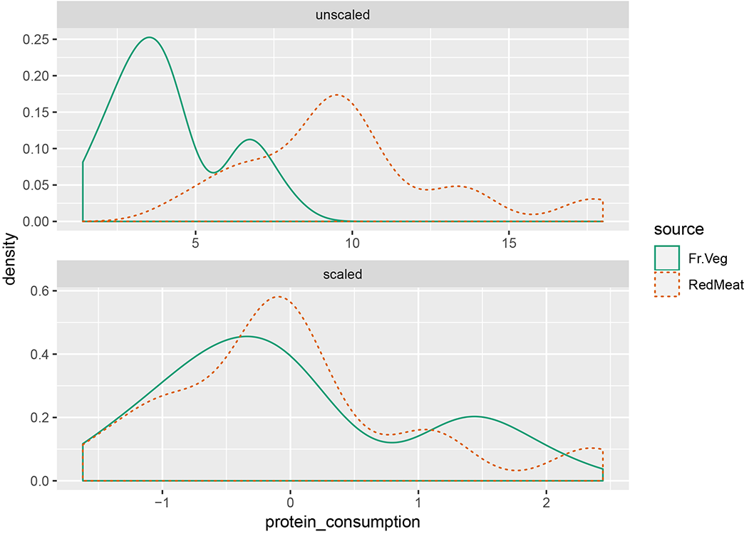
Figure 9.6. Dendrogram of countries clustered by protein consumption
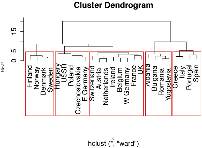
Figure 9.7. The idea behind principal components analysis
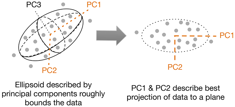
Figure 9.8. Plot of countries clustered by protein consumption, projected onto first two principal components
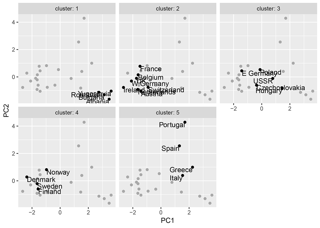
Figure 9.9. Jaccard similarity
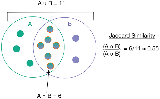
Figure 9.10. Cluster WSS and total WSS for a set of four clusters
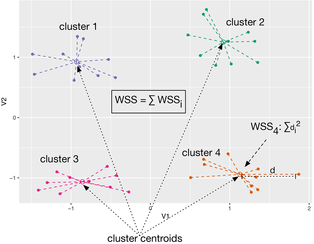
Figure 9.11. WSS as a function of k for the protein data
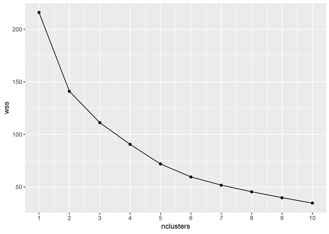
Figure 9.12. Total sum of squares (TSS) for a set of four clusters
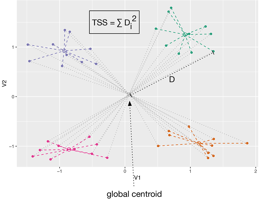
Figure 9.13. BSS and WSS as a function of k
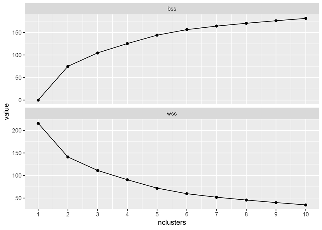
Figure 9.14. The Calinski-Harabasz index as a function of k
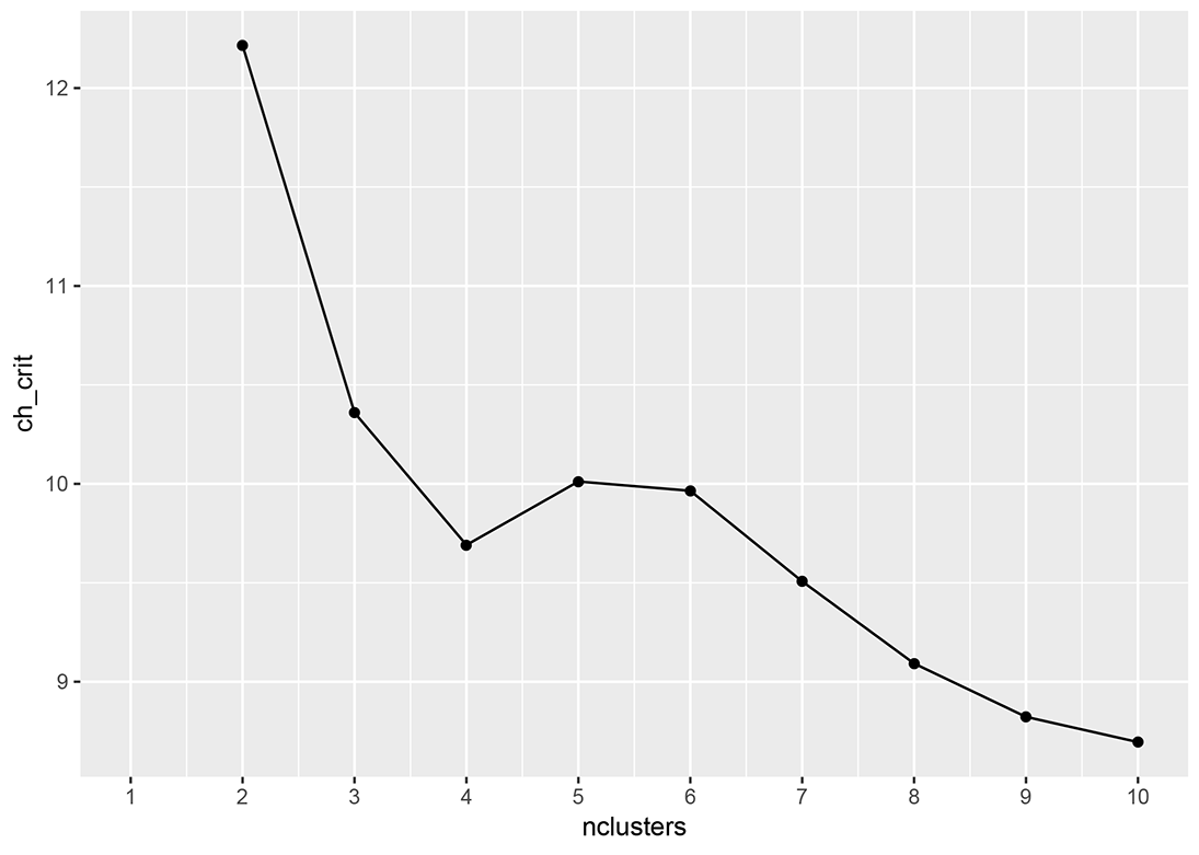
Figure 9.15. The protein data dendrogram with two clusters
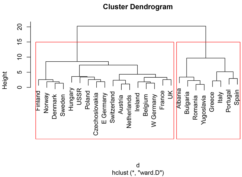
Figure 9.16. The k-means procedure. The two cluster centers are represented by the outlined star and diamond.
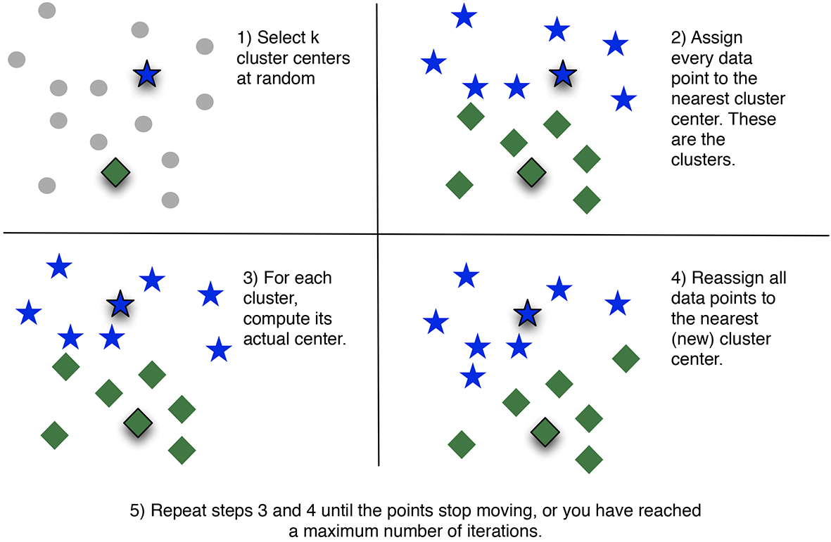
Figure 9.17. Top: Comparison of the (scaled) CH and average silhouette width indices for kmeans clusterings. Bottom: Comparison of CH indices for kmeans and hclust clusterings.
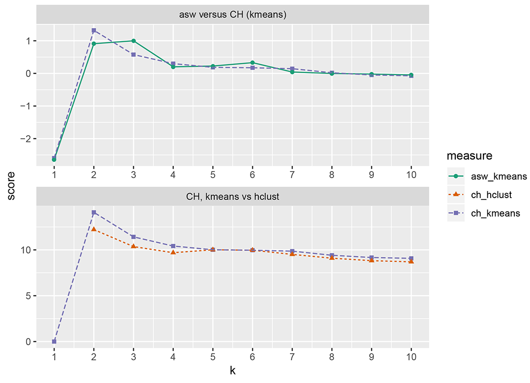
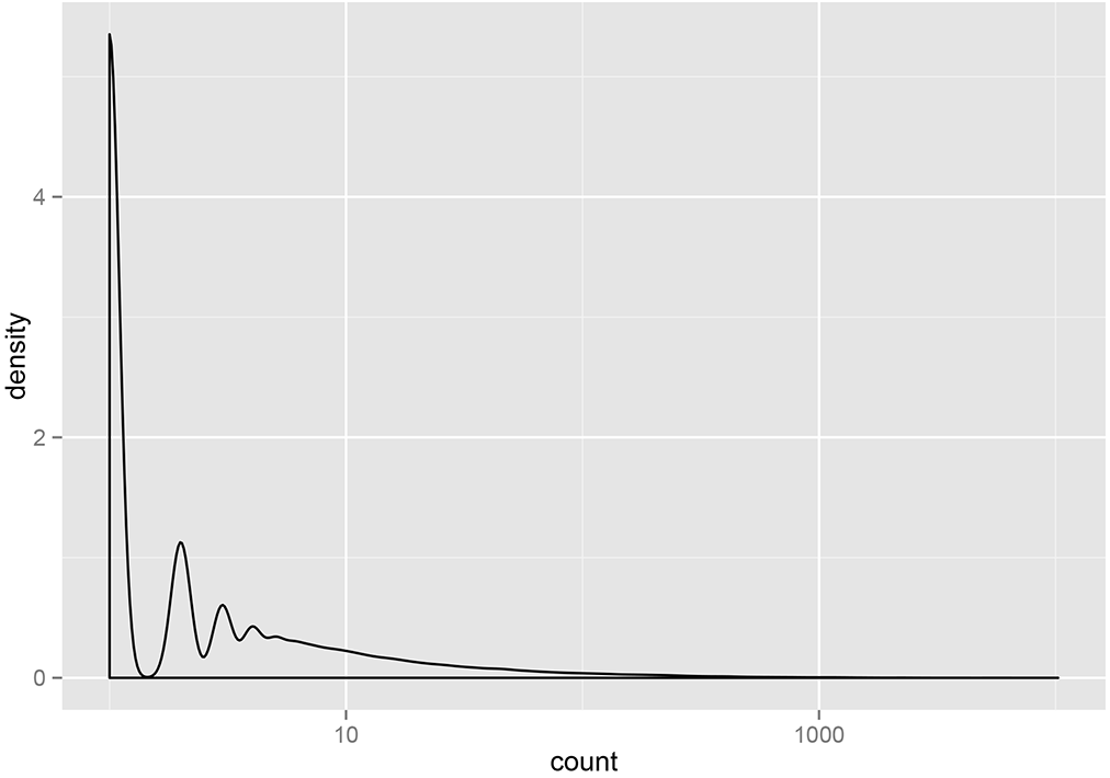
Figure 9.18. A density plot of basket sizes
Summary
In this chapter, you’ve learned how to find similarities in data using two different clustering methods in R, and how to find items that tend to occur together in data using association rules. You’ve also learned how to evaluate your discovered clusters and your discovered rules.
Unsupervised methods like the ones we’ve covered in this chapter are really more exploratory in nature. Unlike with supervised methods, there’s no “ground truth” to evaluate your findings against. But the findings from unsupervised methods can be the starting point for more focused experiments and modeling.
In the last few chapters, we’ve covered the most basic modeling and data analysis techniques; they’re all good first approaches to consider when you’re starting a new project. In the next chapter, we’ll touch on a few more advanced methods.
In this chapter you learned:
- How to cluster unlabelled data using both hierarchical methods and k-means.
- How to estimate what the appropriate number of clusters should be.
- How to evaluate an existing clustering for cluster stability.
- How to find patterns (association rules) in transaction data using apriori.
- How to evaluate and sort through discovered association rules.
FAQ
What are “unsupervised methods” and when should I use them?
Unsupervised methods discover structure without a target outcome. They’re exploratory tools to reveal patterns you didn’t pre-specify—such as groups of similar records (clustering) or items that co-occur (association rules). Treat them as modeling steps you still evaluate, and often as precursors to supervised learning.How do I choose an appropriate distance or similarity for clustering?
- Euclidean: default for quantitative, real-valued features; basis of k-means (squared Euclidean).- Manhattan (L1): when “street-block” movement or robustness to outliers matters.
- Hamming: for purely categorical/indicator features (counts mismatches).
- Cosine similarity: for high-dimensional sparse nonnegative vectors (e.g., text); convert to a distance via 1 − cosine or a proper angle-based metric.
Ordered categories can be mapped to numbers before using quantitative distances.
Why does scaling matter, and how do I scale data in R before clustering?
Distances are unit-dependent; variables with larger scales can dominate clustering. Standardize each numeric column to mean 0 and standard deviation 1 (e.g., with R’s scale()). Save the attributes scaled:center and scaled:scale so you can consistently transform new data and, if needed, “unscale” results.How do I run hierarchical clustering in R and interpret the dendrogram?
Compute a distance matrix (dist(), e.g., method = "euclidean"), then hclust() (e.g., method = "ward.D"). Plot the dendrogram to see nested groupings. Choose a number of clusters by “cutting” the tree (rect.hclust(), then cutree() to extract labels). Nearby leaves that connect at low heights belong together.What’s a simple way to visualize clusters from high-dimensional data?
Project data to the first two principal components (prcomp(); predict()) and plot PC1 vs PC2, optionally faceted or colored by cluster. This 2D view captures as much variance as possible in two axes and often reveals separation or overlap between clusters.How can I pick a good number of clusters k?
Try multiple heuristics and compare: (1) Elbow in total within sum of squares (WSS) vs k; (2) Calinski–Harabasz (CH) index, maximizing between-cluster separation relative to within-cluster spread; (3) Gap statistic (works best for mixtures of Gaussians); (4) Average silhouette width. Use domain knowledge and validate choices rather than relying on a single rule.How do I assess whether clusters are “real” (stable)?
Use bootstrap stability via fpc::clusterboot(). It re-clusters bootstrap samples and scores each original cluster by the Jaccard coefficient with its best match. Rule of thumb: stability < 0.6 (unstable), 0.6–0.75 (some signal, uncertain membership), > 0.85 (highly stable). Note stability also depends on the clustering algorithm.What should I know about k-means in practice?
- Works on numeric data with squared Euclidean distance; often best for roughly Gaussian, spherical clusters.- Sensitive to initialization; run multiple random starts (nstart) and pick the lowest total WSS.
- Not guaranteed unique; compare solutions and k via CH, silhouette, or stability checks.
- Returns centers, sizes, and sums of squares for evaluation.
How do I assign new points to existing clusters correctly?
Standardize the new point using the same center/scale used for training. Compute its (squared Euclidean) distance to each cluster centroid and assign it to the nearest one. Keep and reuse the original scaling parameters and the learned centroids.How do I mine and evaluate association rules with arules in R?
- Concepts: a transaction is a “basket”; items form itemsets. Support = fraction of transactions containing an itemset; confidence = P(Y|X); lift = support(X,Y) / (support(X)·support(Y)).- Workflow: read.transactions(), set low but reasonable support (high-dimensional data makes most items rare) and confidence, then apriori(). Use inspect() and sort() to review rules.
- Evaluate: interestMeasure() for coverage (support of lhs) and fishersExactTest (small p-values indicate non-random co-occurrence). Use appearance to constrain rhs/lhs (e.g., rules predicting a specific item). Iterate by filtering and re-scoring to find actionable rules.

 Practical Data Science with R, Second Edition ebook for free