Overview

7 Linear and logistic regression

This chapter moves from model evaluation to model building, showing how to fit, interpret, and stress-test linear and logistic regression in R. It treats both methods as tools for prediction and for extracting actionable advice from coefficients, while emphasizing careful diagnostics, out-of-sample checks, and the dangers of extrapolation. Along the way it highlights common pitfalls such as collinearity for linear models and separation for logistic models, and motivates regularization as a principled remedy. The overall message is pragmatic: start simple, inspect assumptions and errors, validate on test data, and tune models to be both reliable and interpretable in production.

For predicting numeric outcomes, the chapter presents linear regression with lm, framing the target as a linear combination of inputs plus unsystematic noise that yields unbiased averages and good totals. Using an income example, it demonstrates training, prediction, and quality checks via true-vs-predicted plots, residual plots, R-squared, and RMSE, and it explains how to read summary(model): residual distributions, coefficient estimates and p-values, degrees of freedom, residual standard error, adjusted R-squared, and the F-test. It shows how to interpret coefficients for continuous and categorical variables (reference levels, indicator coding, intercept meaning), and warns that correlated inputs can inflate magnitudes, flip signs, and undermine coefficient-level “advice” even when predictions remain acceptable. The guidance is to trust only statistically significant coefficients, beware high standard errors and unexpected signs, and rely on test-set performance as the final safeguard.

For probabilities and binary classification, the chapter introduces logistic regression with glm (binomial logit), deriving it as a linear model on log-odds with the sigmoid mapping back to probabilities. A neonatal risk case study illustrates training, calibrated predictions (summing to observed positives), and performance analysis using score distributions, precision–recall trade-offs, enrichment, threshold selection, and confusion matrices. It covers coefficient interpretation as odds multipliers, pseudo R-squared from null and residual deviance, chi-squared tests for model significance, AIC for model choice, and Fisher scoring iterations as a convergence diagnostic; it also cautions about separation and quasi-separation. To stabilize estimates and improve generalization under collinearity or separation, the chapter introduces regularization via glmnet: ridge (L2) to “share credit,” lasso (L1) to select variables by zeroing coefficients, and elastic net to blend both, with cross-validation to choose lambda (and alpha), standardization by default, and the reminder that regularization slightly alters coefficient interpretability while often yielding safer, more robust models.

Figure 7.1. Mental model
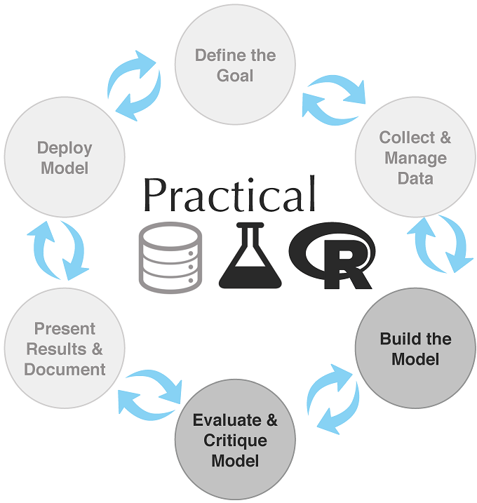
Mental model
Figure 7.2. The linear relationship between daily_cals_down and daily_exercise
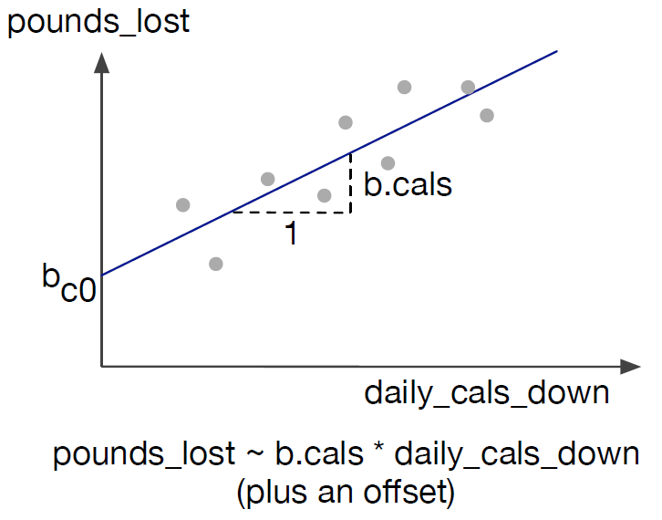
The linear relationship between daily_cals_down and daily_exercise
Figure 7.3. pounds_lost as a linear combination of daily_exercise and daily_cals_down
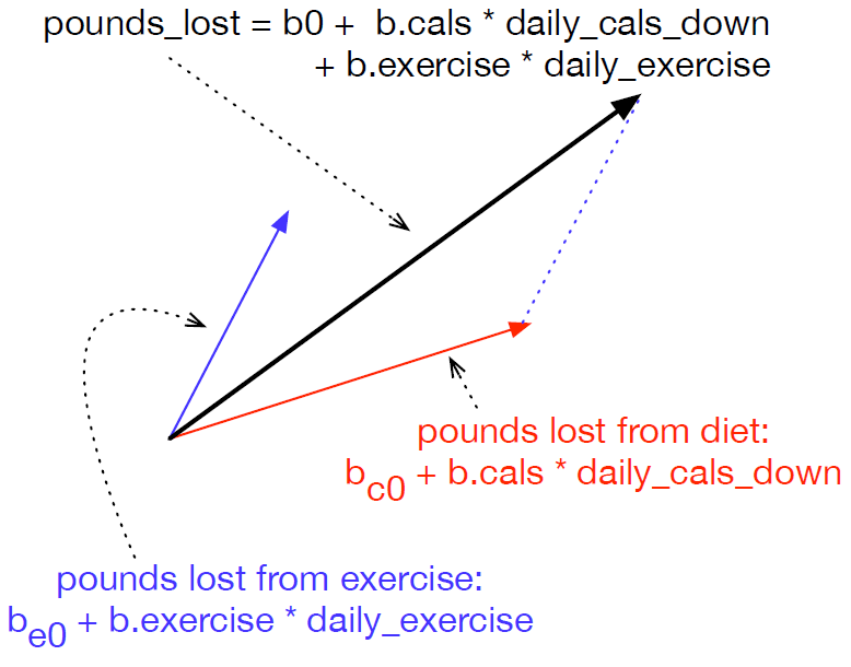
pounds_lost as a linear combination of daily_exercise and daily_cals_down
Figure 7.4. Fit versus actuals for y=x^2
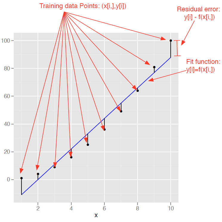
Fit versus actuals for y=x^2
Figure 7.5. Building a linear model using the lm() command
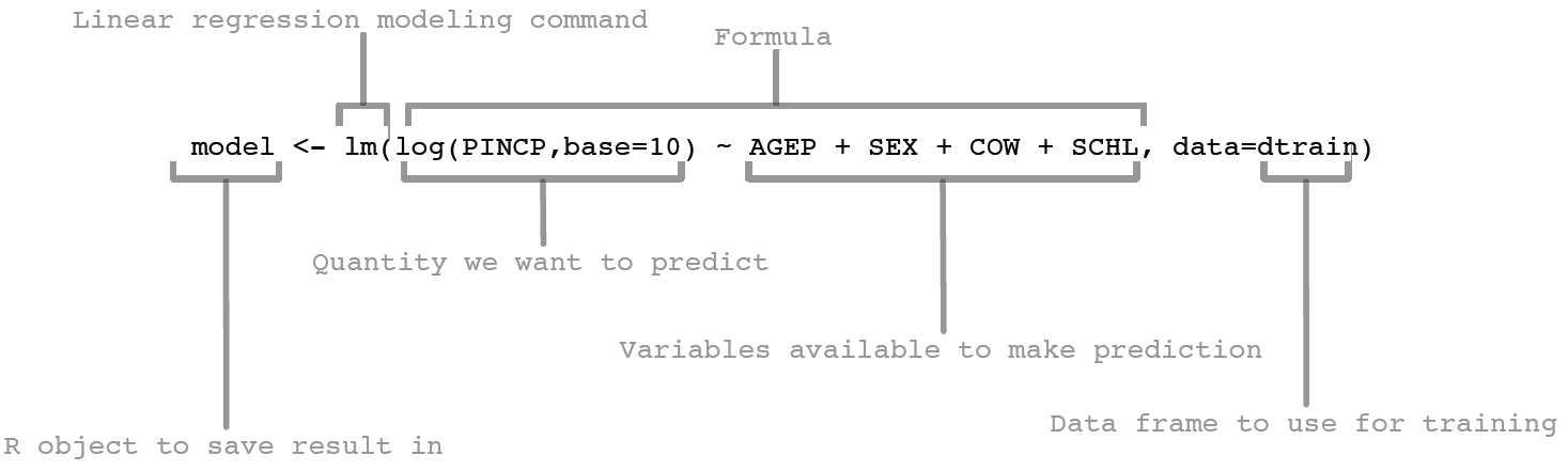
Building a linear model using the lm() command
Figure 7.6. Making predictions with a linear regression model
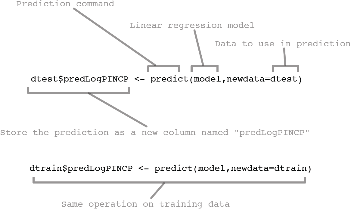
Making predictions with a linear regression model
Figure 7.7. Plot of actual log income as a function of predicted log income
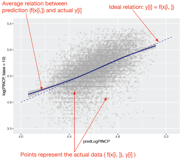
Plot of actual log income as a function of predicted log income
Figure 7.8. Plot of residual error as a function of prediction
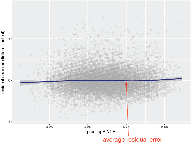
Plot of residual error as a function of prediction
Figure 7.9. An example of systematic errors in model predictions
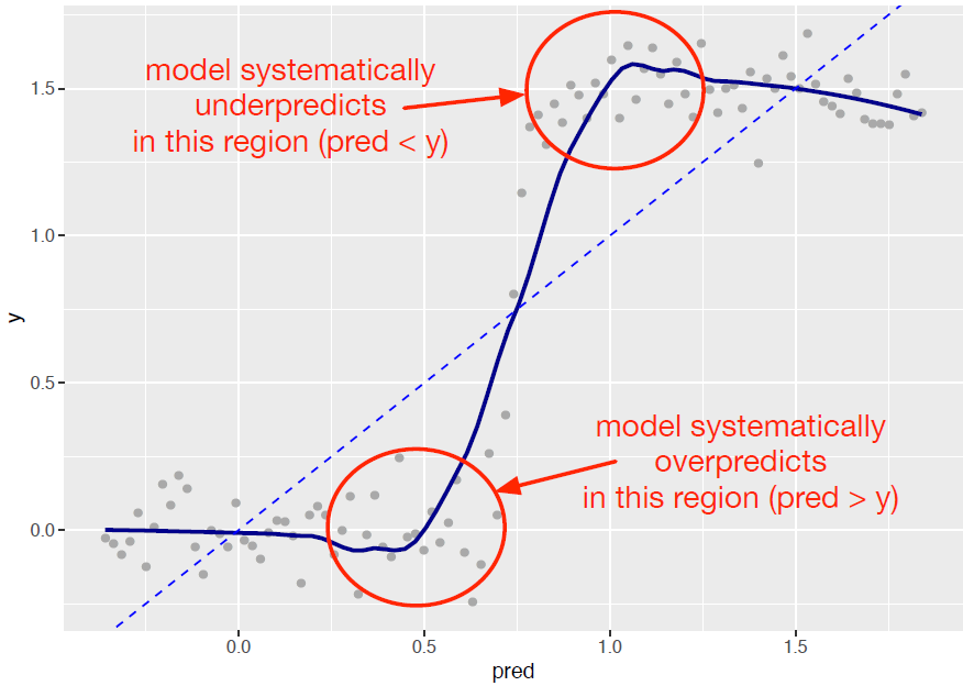
An example of systematic errors in model predictions
Figure 7.10. The model coefficients
The model coefficients
Figure 7.11. Model summary
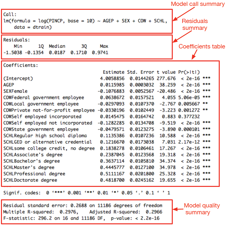
Model summary
Figure 7.12. Model summary coefficient columns
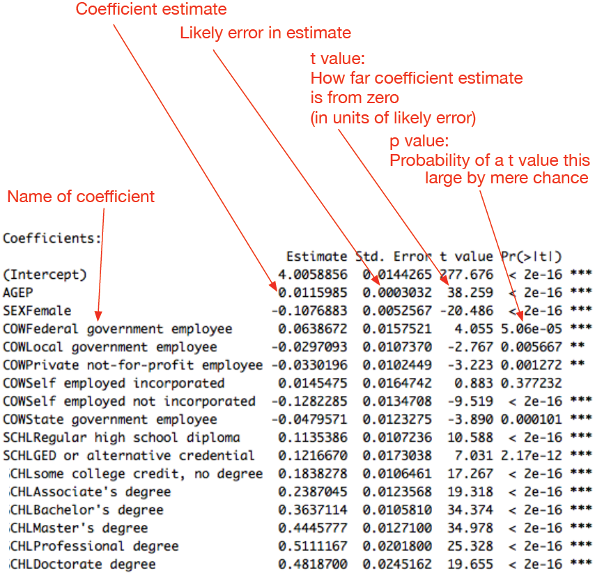
Model summary coefficient columns
Figure 7.13. Mapping the odds of a flight delay to the log-odds
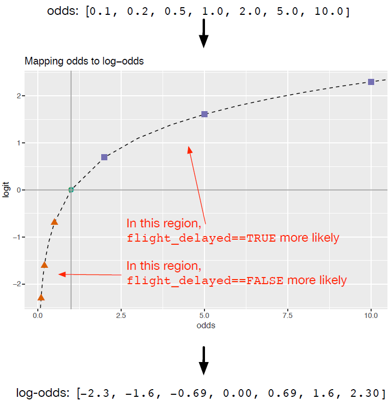
Mapping the odds of a flight delay to the log-odds
Figure 7.14. Mapping log-odds to the probability of a flight delay via the sigmoid function
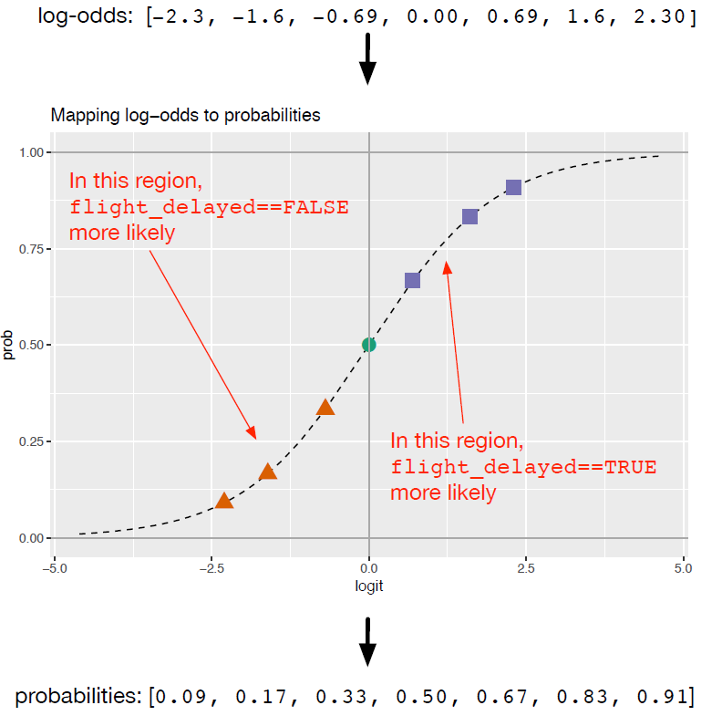
Mapping log-odds to the probability of a flight delay via the sigmoid function
Figure 7.15. Distribution of score broken up by positive examples (TRUE) and negative examples (FALSE)
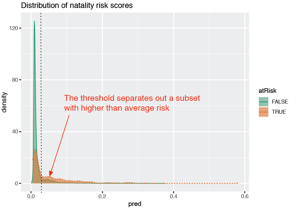
Distribution of score broken up by positive examples (TRUE) and negative examples (FALSE)
Figure 7.16. Reproduction of the spam filter score distributions from chapter 6
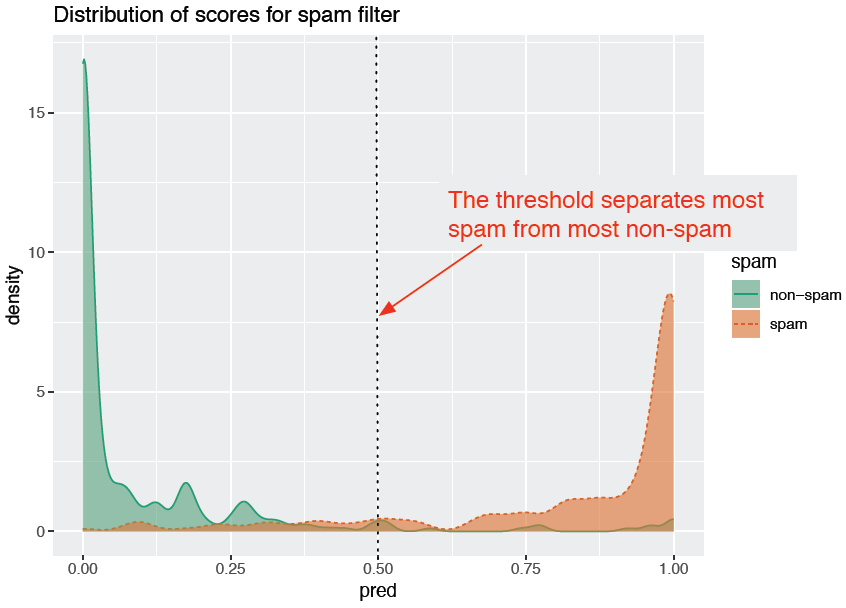
Reproduction of the spam filter score distributions from chapter 6
Figure 7.17. Enrichment (top) and recall (bottom) plotted as a functions of threshold for the training set
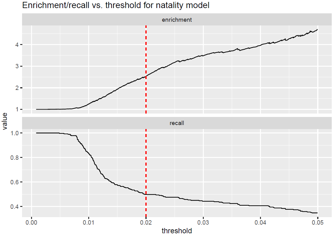
Enrichment (top) and recall (bottom) plotted as a functions of threshold for the training set
Figure 7.18. Coefficients of the logistic regression model
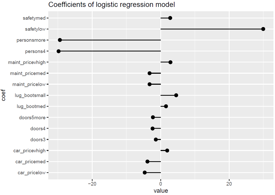
Coefficients of the logistic regression model
Figure 7.19. Schematic of cv.glmnet()
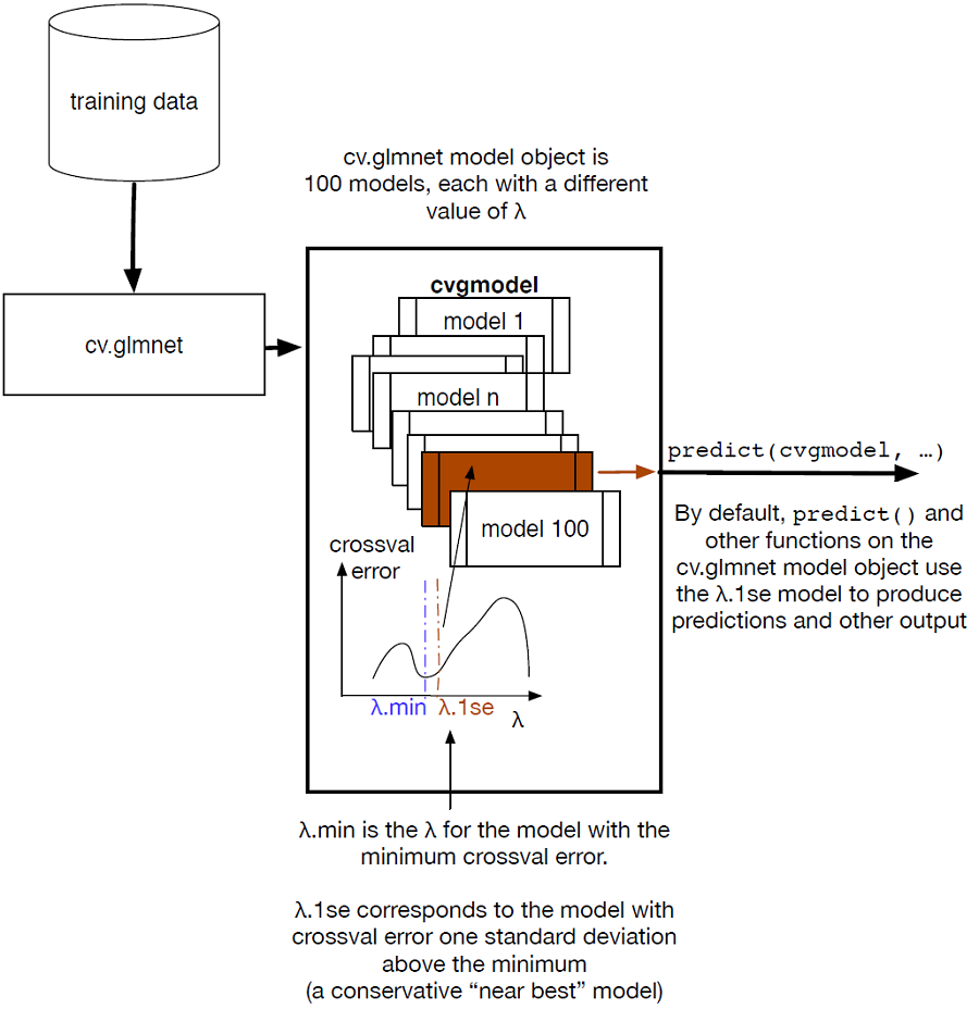
Schematic of cv.glmnet()
Figure 7.20. Coefficients of the ridge regression model
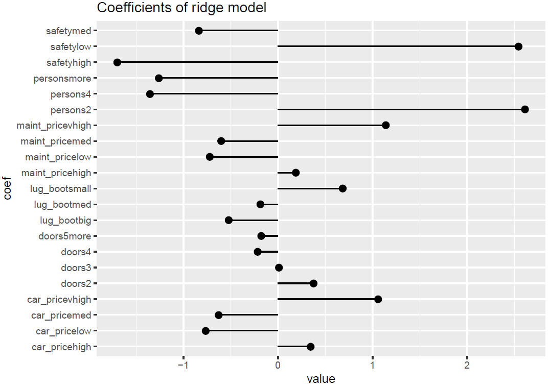
Coefficients of the ridge regression model
Figure 7.21. Coefficients of the lasso regression model
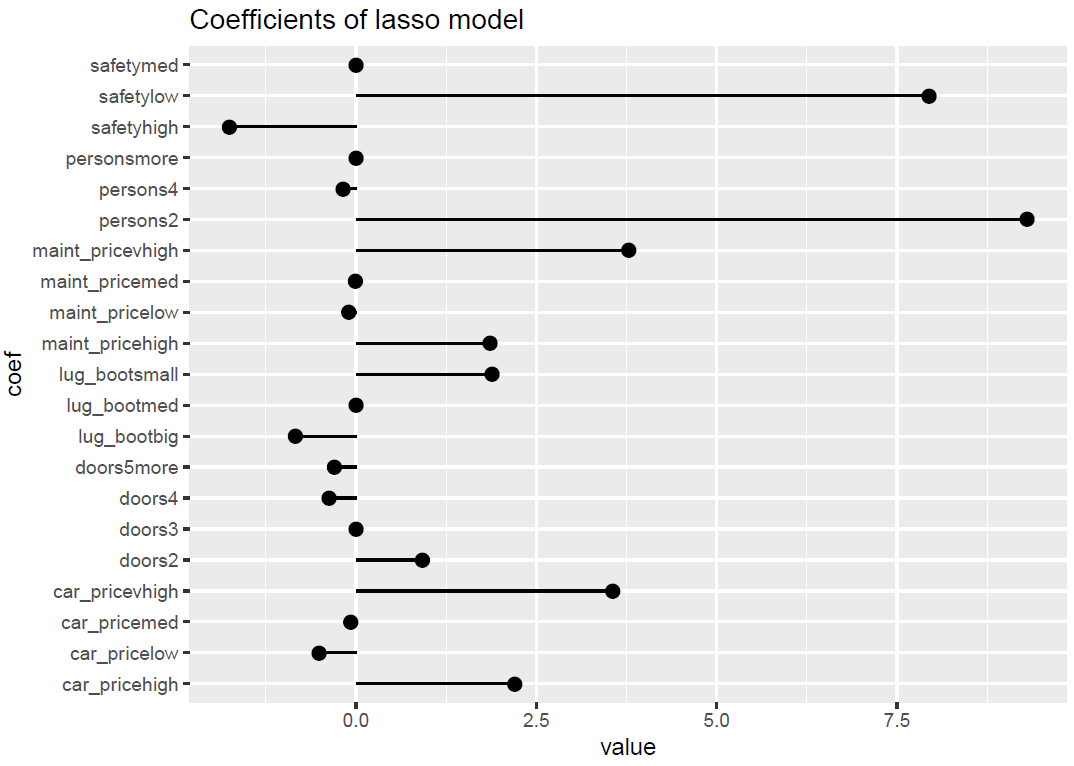
Coefficients of the lasso regression model
Figure 7.22. Schematic of using cva.glmnet to pick alpha
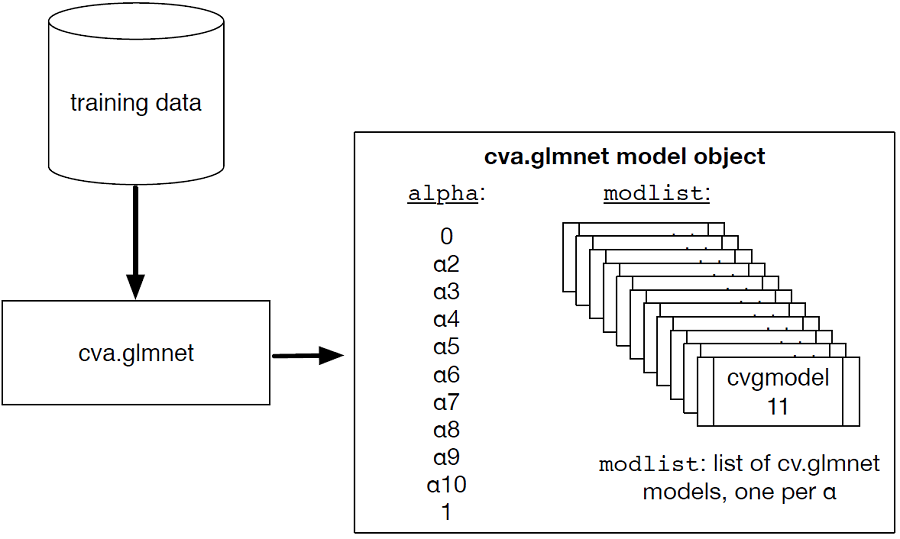
Schematic of using cva.glmnet to pick alpha
Figure 7.23. Cross validation error as a function of alpha
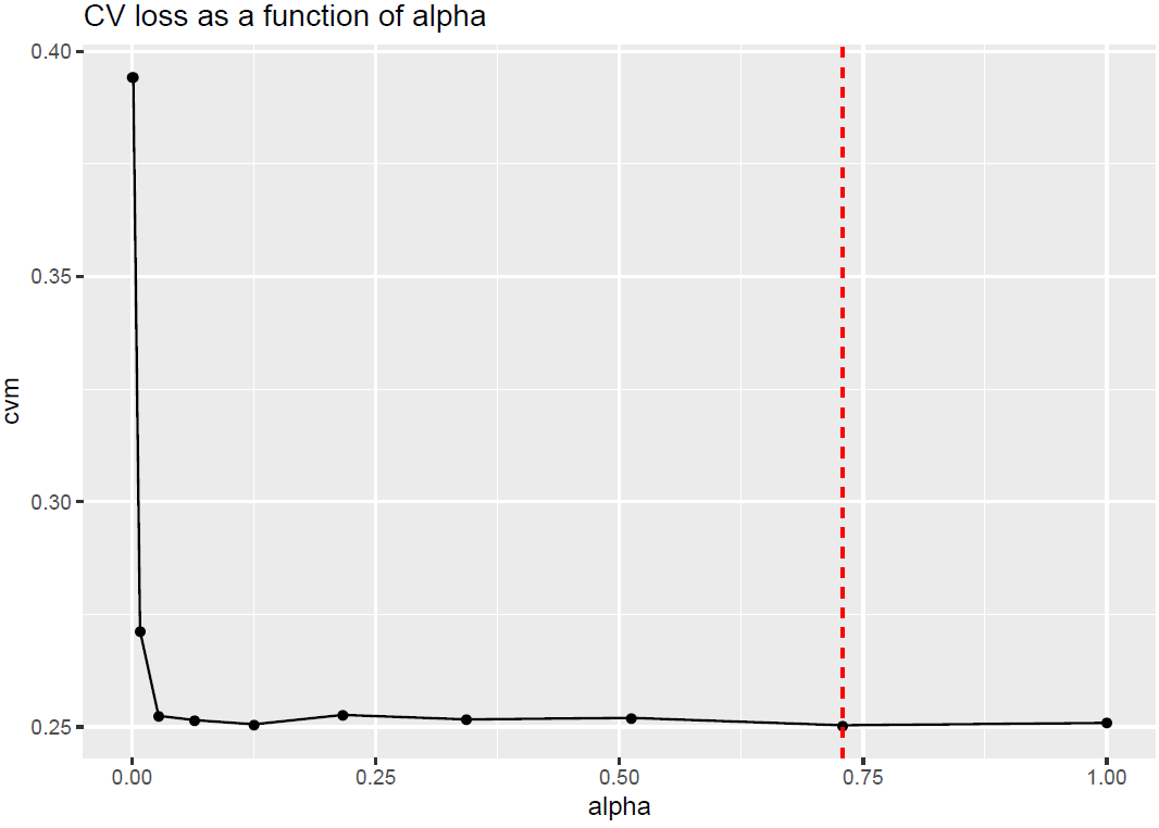
Cross validation error as a function of alpha

 Summary

Both linear and logistic regression assume that the outcome is a function of a linear combination of the inputs. This seems restrictive, but in practice linear and logistic regression models can perform well even when the theoretical assumptions aren’t exactly met. We’ll show how to further work around these limits in chapter 10.

Linear and logistic regression can also provide advice by quantifying the relationships between the outcomes and the model’s inputs. Since the models are expressed completely by their coefficients, they’re small, portable, and efficient—all valuable qualities when putting a model into production. If the model’s errors are uncorrelated with y, the model might be trusted to extrapolate predictions outside the training range. Extrapolation is never completely safe, but it’s sometimes necessary.

In situations where variables are correlated or the prediction problem is quasi-separable, linear methods may not perform as well. In these cases, regularization methods can produce models that are safer to apply to new data, although the coefficients of these models are not as useful for advice about the relationships between variables and the outcome.

While learning about linear models in this chapter, we have assumed that the data is well-behaved: the data had no missing values, the number of possible levels for categorical variables were low, and all possible levels were present in the training data. In real-world data, these assumptions are not always true. In the next chapter, you will learn about advanced methods to prepare ill-behaved data for modeling.

In this chapter you have learned:

  • How to predict numerical quantities with linear regression models.
  • How to predict probabilities or classify using logistic regression models.
  • How to interpret the diagnostics from lm() and glm() models.
  • How to interpret the coefficients of linear models.
  • How to diagnose when a linear model may not be "safe" or not as reliable (collinearity, quasi-separation).
  • How to use glmnet to fit regularized linear and logistic regression models.

FAQ

When should I start with linear regression, and what are its key assumptions?Use linear regression first when predicting a numeric quantity (for example, income). It assumes the outcome is a linear combination of inputs plus unsystematic noise (mean 0, uncorrelated with inputs). It often predicts well even when reality is only approximately linear, but expect systematic errors if the true relationship is strongly nonlinear or if you extrapolate far outside the training range.
How do I interpret coefficients in a linear regression, including categorical variables?Each coefficient is the expected change in the outcome for a one-unit increase in that input (holding others fixed). For categorical variables, R creates indicators relative to a reference level; each reported level’s coefficient is the difference from that reference. For example, a coefficient of 0.36 on SCHL=“Bachelor’s degree” (with “no high school diploma” as reference) means predicted income on the log10 scale is higher by 0.36; the income ratio is about 10^0.36 ≈ 2.29.
What do the main lm() diagnostics mean (residuals, R-squared, adjusted R-squared, F-statistic)?Residuals summarize errors; you want them centered near 0 with no strong pattern. R-squared is the fraction of variance explained; adjusted R-squared penalizes extra variables and is preferred when you lack a test set. The F-statistic (with a small p-value) shows the model explains more variance than a constant-only model.
How should I check prediction quality for a linear model?Plot actuals vs predictions (look for points near the y=x line) and residuals vs predictions (look for a band around 0 without structure). Compute R-squared on both train and test (similar values suggest no overfit) and RMSE (lower is better). Large systematic curves in residuals suggest a nonlinear method may be better.
What is logistic regression and how do I interpret its coefficients?Logistic regression models P(y=1) = sigmoid(a + b·x), i.e., it fits a linear model on log-odds. A coefficient b[k] multiplies the odds by exp(b[k]) per unit increase in x_k. Positive b increases odds (and probability) of the target class; negative b decreases it. Use glm(..., family=binomial(link="logit")).
How do I make probability predictions with glm(), and why type="response"?Use predict(model, newdata=..., type="response") to return probabilities (not log-odds). A useful property: logistic regression preserves marginal probabilities on the training set—the sum of predicted probabilities equals the number of positives (and similarly within subgroups defined by model inputs).
How do I assess logistic model quality (deviance, pseudo R-squared, AIC, significance)?Null deviance is fit of an intercept-only model; residual deviance is fit of your model (lower is better). Pseudo R-squared = 1 − (resid.dev/null.dev) gauges goodness-of-fit (higher is better). AIC balances fit and complexity (lower is better when comparing models on the same data). A chi-squared test on the deviance reduction (small p-value) indicates the model improves over the null.
What can go wrong with lm()/glm(), and what are the warning signs?Collinearity (correlated inputs) inflates coefficient magnitudes and standard errors, can flip signs, and lowers coefficient significance in both lm() and glm(). In logistic regression, separation or quasi-separation (some inputs perfectly predict outcomes in a subset) causes non-convergence, huge coefficients with huge SEs, warnings like “fitted probabilities 0 or 1,” and many Fisher scoring iterations.
What is regularization (ridge, lasso, elastic net), and when should I use each?Regularization penalizes large coefficients to improve stability and generalization. Ridge (L2) shrinks and “shares credit” among correlated variables; useful for collinearity and quasi-separation. Lasso (L1) can shrink some coefficients exactly to zero (feature selection). Elastic net blends both (alpha between 0 and 1) to combine their benefits.
How do I fit regularized models in R with glmnet, and choose lambda/alpha?Use glmnetUtils::cv.glmnet(formula, data, family="binomial" or "gaussian", alpha=...) for cross-validated lambda; by default, use lambda.1se for a simpler model. For elastic net, use glmnetUtils::cva.glmnet(...) to search alpha and lambda, then refit with cv.glmnet at the chosen alpha. Note glmnet standardizes inputs by default and expands all factor levels (no single reference level).

pro $24.99 per month

  • access to all Manning books, MEAPs, liveVideos, liveProjects, and audiobooks!
  • choose one free eBook per month to keep
  • exclusive 50% discount on all purchases
  • renews monthly, pause or cancel renewal anytime

lite $19.99 per month

  • access to all Manning books, including MEAPs!

team

5, 10 or 20 seats+ for your team - learn more


choose your plan

team

monthly
annual
$49.99
$499.99
only $41.67 per month
  • five seats for your team
  • access to all Manning books, MEAPs, liveVideos, liveProjects, and audiobooks!
  • choose another free product every time you renew
  • choose twelve free products per year
  • exclusive 50% discount on all purchases
  • renews monthly, pause or cancel renewal anytime
  • renews annually, pause or cancel renewal anytime
  • Practical Data Science with R, Second Edition ebook for free

choose your plan

team

monthly
annual
$49.99
$499.99
only $41.67 per month
  • five seats for your team
  • access to all Manning books, MEAPs, liveVideos, liveProjects, and audiobooks!
  • choose another free product every time you renew
  • choose twelve free products per year
  • exclusive 50% discount on all purchases
  • renews monthly, pause or cancel renewal anytime
  • renews annually, pause or cancel renewal anytime
  • Practical Data Science with R, Second Edition ebook for free