6 Choosing and evaluating models
This chapter presents a practical roadmap for the modeling workflow: start by translating business questions into machine learning tasks, then choose methods that match your intended use, and finally test and explain your results. It distinguishes three broad problem families you will encounter: classification (assigning labels), scoring or regression (predicting numbers or probabilities), and grouping via unsupervised learning (discovering structure without known targets). Typical choices include logistic regression and decision trees for classification, regression models for numeric targets or probabilities, and techniques like k-means clustering and association rules for pattern discovery. The guidance emphasizes picking approaches that align with how the model will be used—for example, regression to quantify variable effects, or tree-based methods to uncover dominant decision drivers—and recognizing when multiclass settings require methods beyond simple two-class setups.
To ensure models generalize, the chapter stresses disciplined evaluation. Split data into training and hold-out sets to detect overfitting and guard against optimistic and multiple-comparison bias; add a calibration set or use k-fold cross-validation when data is limited or during hyperparameter tuning. Always benchmark against simple baselines such as a null model and the best single-variable model. For classifiers, use the confusion matrix to derive accuracy, but prefer precision, recall, F1, and sensitivity/specificity—especially under class imbalance and when threshold choices trade off misses versus false alarms. For scoring models, assess residuals with RMSE and quantify explanatory power with R-squared. For probability models, compare by threshold-independent criteria such as ROC/AUC, and consider log likelihood, deviance, pseudo R-squared, and AIC to balance fit against complexity. Throughout, prefer simpler models when they perform comparably and design evaluation metrics that reflect business costs and benefits.
Finally, the chapter introduces model explainability with LIME, a local, model-agnostic technique that perturbs an example to learn a simple surrogate explaining a complex model’s prediction near that point. LIME helps validate that models rely on meaningful signals (not artifacts), surfaces feature contributions on tabular and text data, and can reveal issues such as sensitivity to class prevalence or unintended bias. Used alongside hold-out testing, LIME supports better stakeholder trust, targeted feature engineering, threshold setting, and fairness checks. The overarching message is to couple the right task framing with rigorous, business-aligned evaluation and clear explanations so models deliver reliable value in production.
Figure 6.1. Mental model

Figure 6.2. Assigning products to product categories
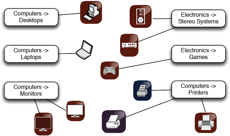
Figure 6.3. Notional example of determining the probability that a transaction is fraudulent
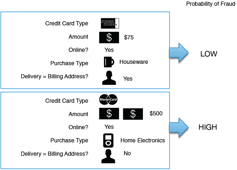
Figure 6.4. Notional example of clustering your customers by purchase pattern and purchase amount
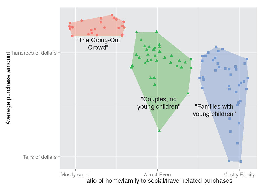
Figure 6.5. Notional example of finding purchase patterns in your data

Figure 6.6. Schematic of model construction and evaluation
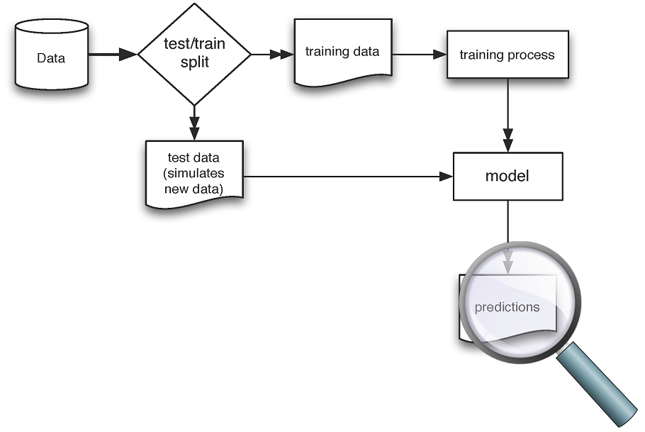
Figure 6.7. A notional illustration of overfitting
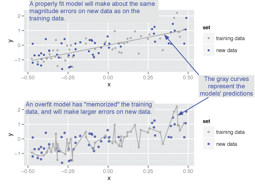
Figure 6.8. Splitting data into training and test (or training, calibration and test) sets
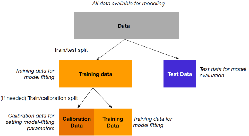
Figure 6.9. Partioning data for 3-fold cross-validation
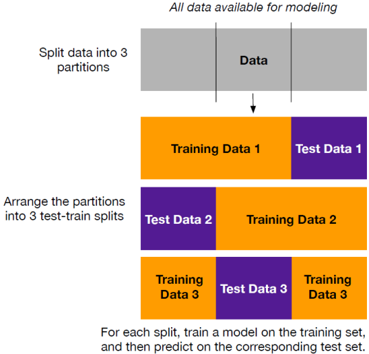
Figure 6.10. Accuracy
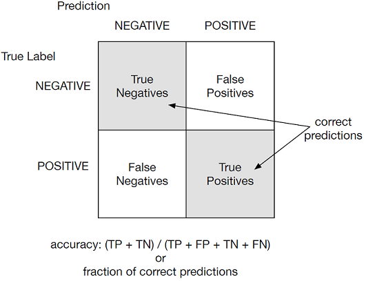
Figure 6.11. Precision
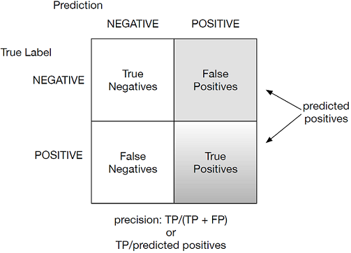
Figure 6.12. Recall
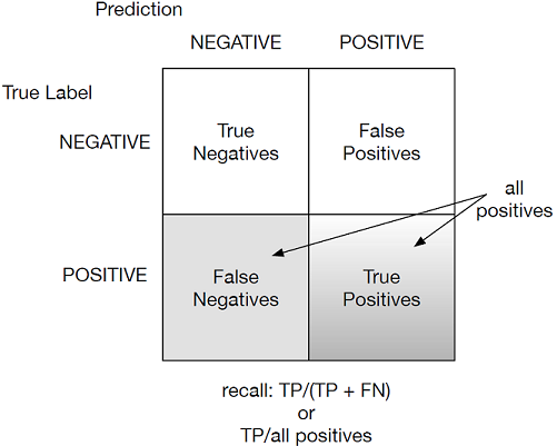
Figure 6.13. Specificity
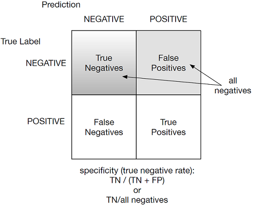
Figure 6.14. Scoring residuals
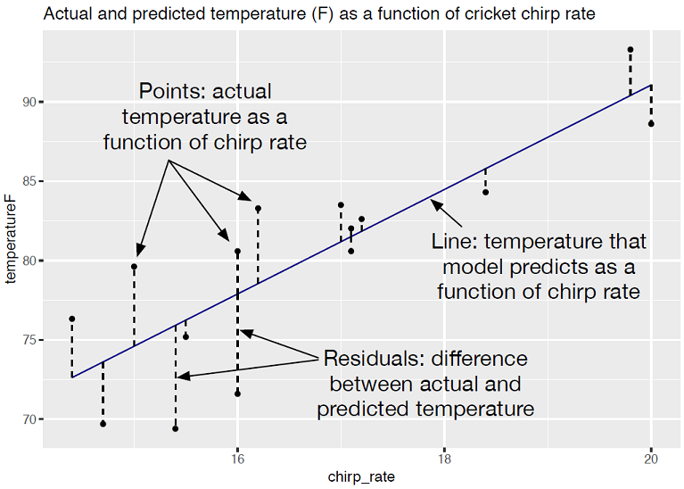
Figure 6.15. Distribution of score broken up by known classes
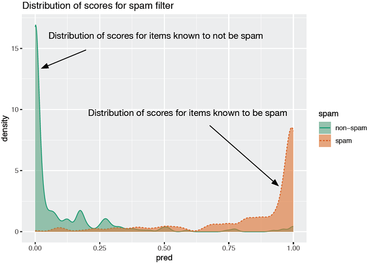
Figure 6.16. ROC curve for the email spam example
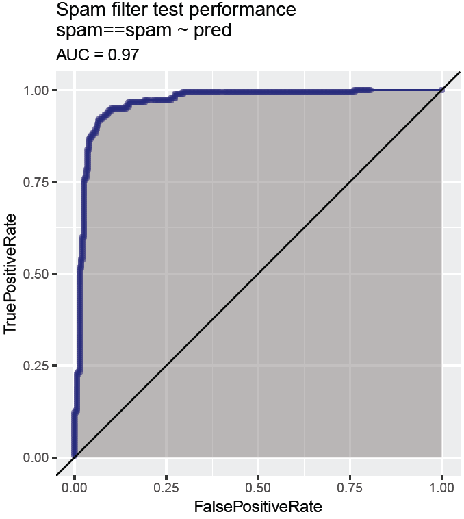
Figure 6.17. ROC curve for an ideal model that classifies perfectly
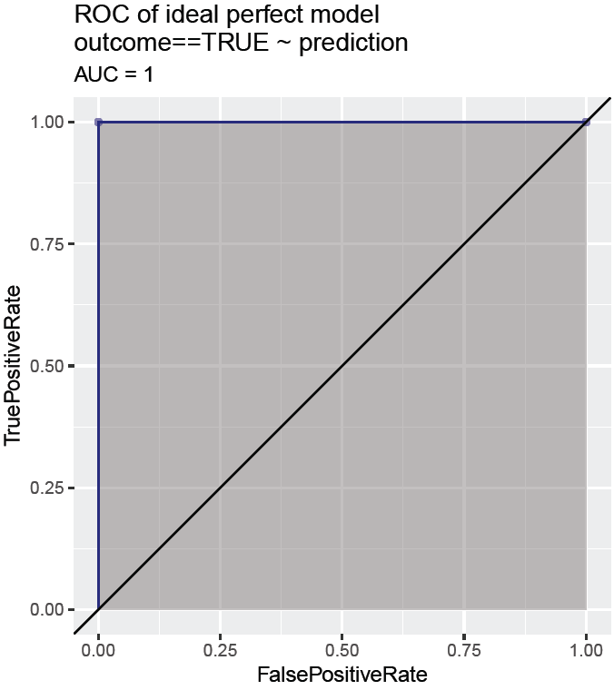
Figure 6.18. Log likelihood of a spam filter prediction
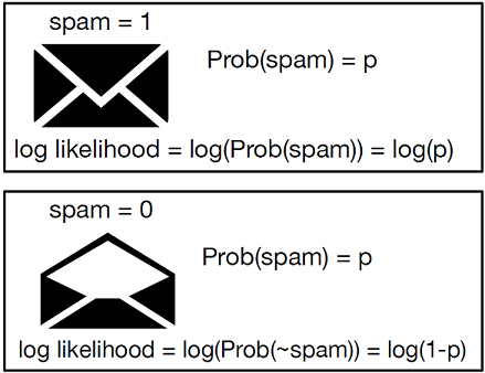
Figure 6.19. Log likelihood penalizes mismatches between the prediction and the true class label
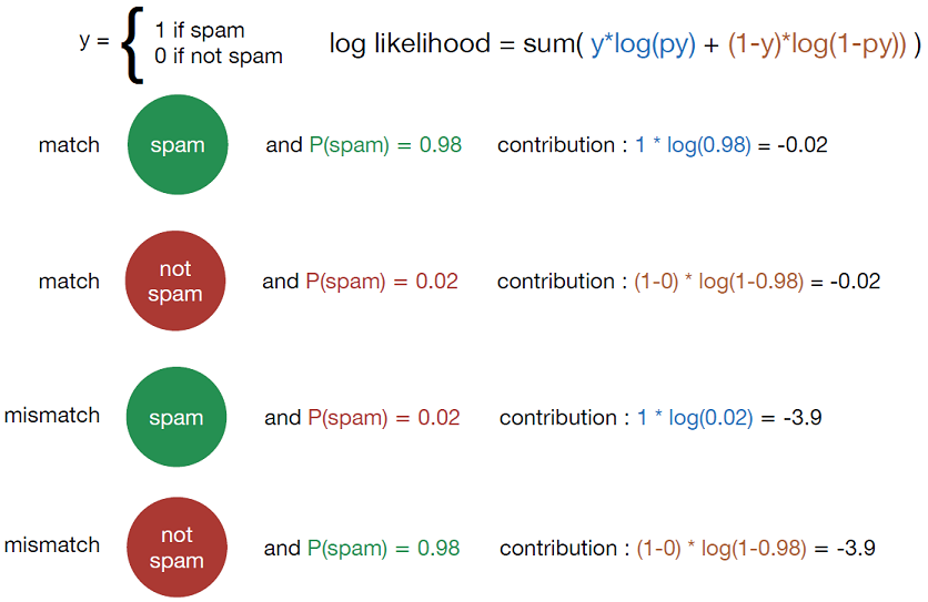
Figure 6.20. Some kinds of models are easier to manually inspect than others
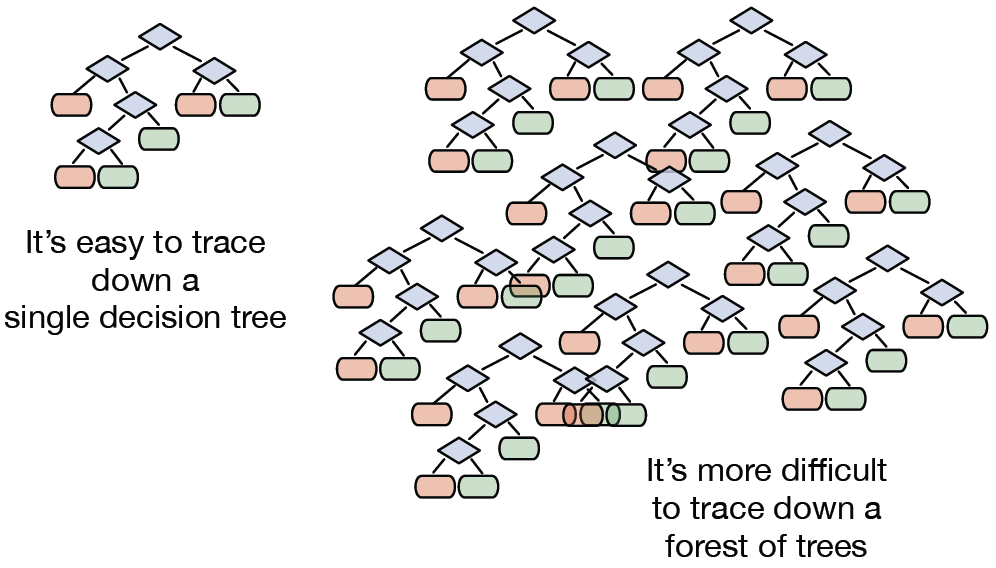
Figure 6.21. Example of a document and the words that most strongly contributed to its classification as "atheist" by the model
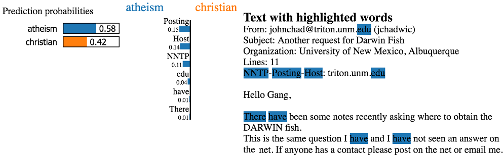
Figure 6.22. Visualize the explanation of the model's prediction
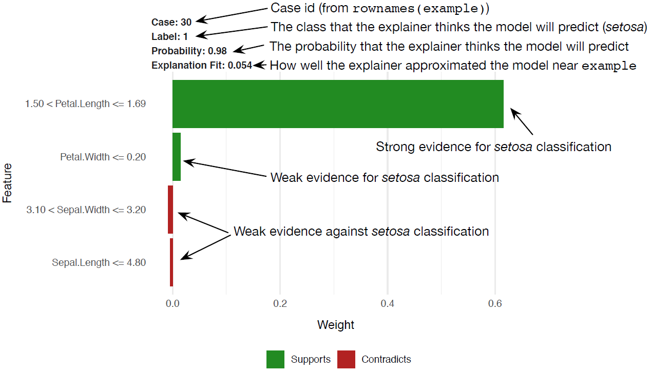
Figure 6.23. Notional sketch of how LIME works
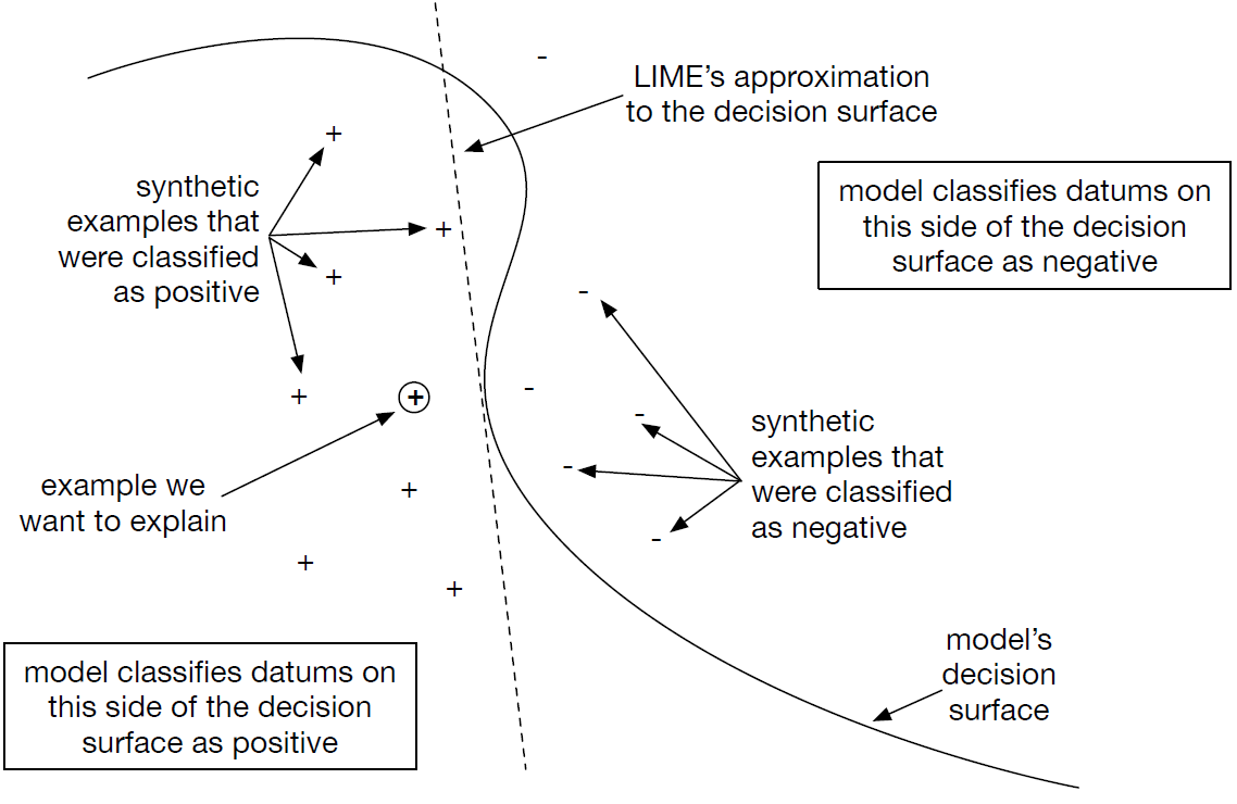
Figure 6.24. Explanations of the two iris examples
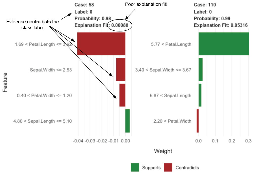
Figure 6.25. Distributions of petal and sepal dimensions by species
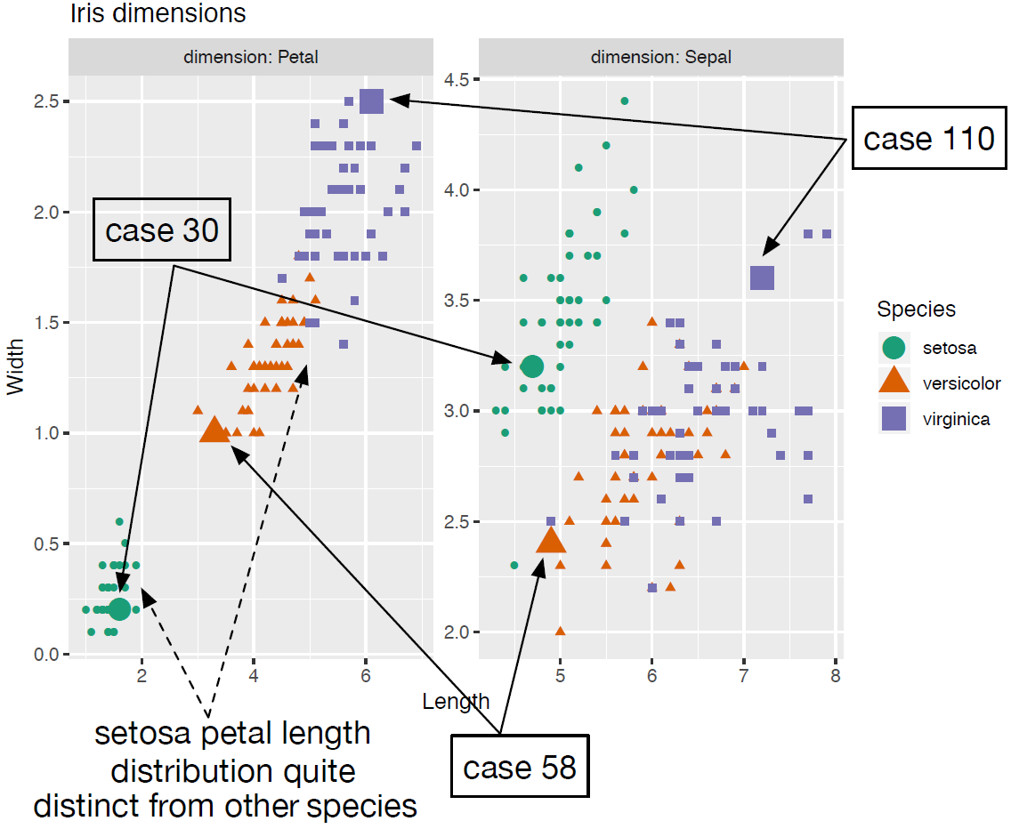
Figure 6.26. Creating a document-term matrix
Figure 6.27. Distribution of test prediction scores
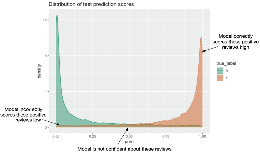
Figure 6.28. Explanation of the prediction on the sample review
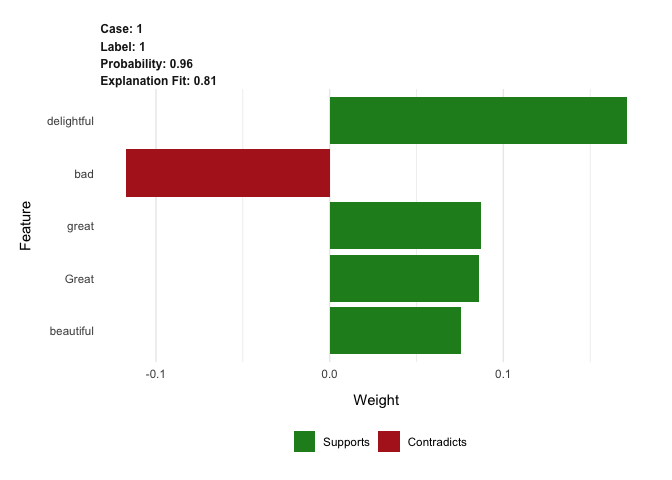
Figure 6.29. Text explanation of the prediction in listing Listing 6.26, “Explain the model's prediction”

Figure 6.30. Explanation visualizations for the two sample reviews Listing 6.27
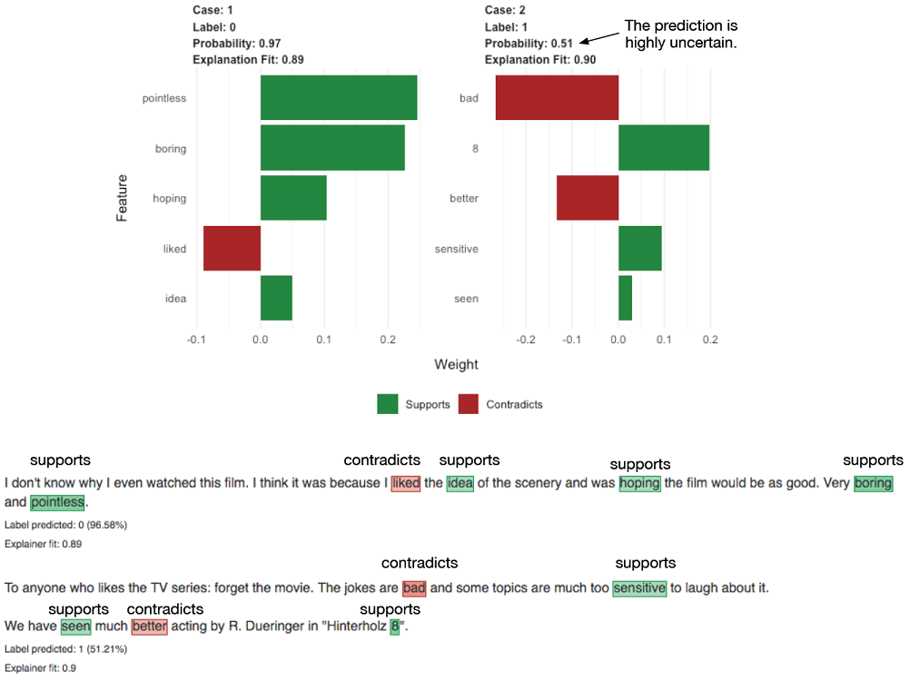
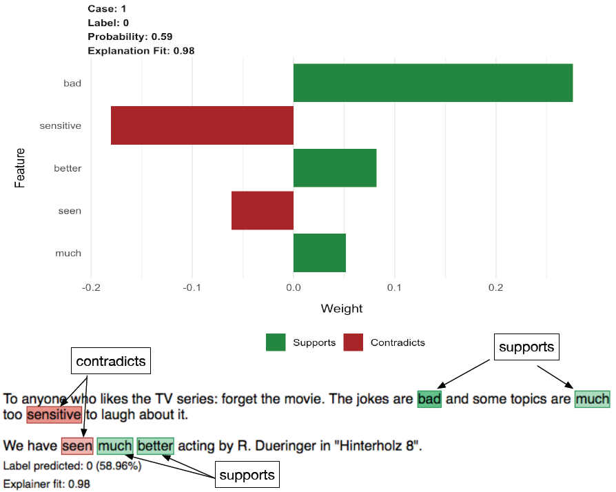
Figure 6.31. Explanation visualizations for the two sample reviews Listing 6.27
Summary
You now have some solid ideas on how to choose among modeling techniques. You also know how to evaluate the quality of data science work, be it your own or that of others. The remaining chapters of part 2 of the book will go into more detail on how to build, test, and deliver effective predictive models. In the next chapter, we’ll actually start building predictive models.
In this chapter you have learned:
- How to match the problem you want to solve to appropriate modeling approaches.
- How to partition your data for effective model evaluation.
- How to calculate various measures for evaluating classification models.
- How to calculate various measures for evaluating scoring (regression) models.
- How to calculate various measures for evaluating probability models.
- How to use the
limepackage to explain individual predictions from a model.
FAQ
How do I map a business problem to the right machine learning task?
Think about the intended use and the form of the output you need:
- Classification: assign labels (for example, spam vs. non-spam, product category).
- Scoring/Regression: predict a numeric value or probability (for example, expected sales uplift, probability of fraud).
- Grouping/Unsupervised: discover structure without known targets (for example, customer segments via clustering, purchase affinities via association rules).
Pick approaches that fit the task and use case. Examples: logistic regression or tree ensembles for classification; linear models or tree ensembles for regression; k-means for clustering; Apriori for association rules.
What is overfitting and how can I detect and mitigate it?
Overfitting happens when a model memorizes training data patterns that don’t generalize. Signs and fixes:
- Detection: large gap between low training error and higher test/hold-out error.
- Mitigation: prefer simpler models, regularize (shrink coefficients), use bagging/ensembles, cross-validate, add more data, reduce leakage, and early-stop iterative learners.
Why split data into training, calibration, and test sets, and what ratios should I use?
Splitting gives an unbiased estimate of future performance and helps prevent decisions based on optimistic training metrics.
- Typical splits: 70/30 or 80/20 train/test; optionally add a calibration/validation set to tune models without touching the final test set.
- Hold back the test set until the end; every choice after seeing test performance introduces bias.
When should I use k-fold cross-validation instead of a simple hold-out?
Use k-fold cross-validation when data is limited or you need more precise performance estimates or to tune hyperparameters.
- k-fold CV trains and evaluates k times on different folds so every example is used for both training and testing (just not simultaneously).
- For large datasets, a simple hold-out is often sufficient and faster.
What is a confusion matrix and which classification metrics come from it?
A confusion matrix tabulates predicted vs. true classes (TP, FP, TN, FN). From it you can compute:
- Accuracy = (TP + TN) / total.
- Precision = TP / (TP + FP): correctness of positive predictions.
- Recall (Sensitivity, TPR) = TP / (TP + FN): coverage of actual positives.
- Specificity (TNR) = TN / (TN + FP): coverage of actual negatives.
- F1 = harmonic mean of precision and recall.
Which baselines should I compare against, and why can accuracy be misleading?
Always beat simple baselines:
- Null model: constant prediction (most common class for classification; mean for regression).
- Best single-variable model: strongest single predictor from your data.
Accuracy can mislead with class imbalance or unequal costs: a model that always predicts the majority class can be “accurate” yet useless. Prefer precision/recall, specificity/sensitivity, or cost-based metrics.
Precision vs. recall vs. F1 vs. sensitivity/specificity: which should I use, and how do I pick a threshold?
Choose metrics that reflect business costs:
- Emphasize precision when false positives are costly (e.g., blocking legit emails).
- Emphasize recall/sensitivity when missing positives is costly (e.g., disease screening).
- Use F1 to balance precision and recall in a single score.
- Specificity complements sensitivity and is prevalence-independent—common in medical testing.
- Pick the classification threshold by exploring trade-offs (ROC/PR curves) and aligning with costs, prevalence, and desired operating points.
How do I evaluate regression (scoring) models?
Common choices:
- RMSE: root mean square error; in the same units as the target; reflects typical prediction error.
- R-squared: fraction of variance explained vs. a null (constant) model; closer to 1 is better.
Report on hold-out/cross-validated data and pair with business thresholds (e.g., “RMSE under $1,000 per account”).
How do I evaluate probability models without fixing a threshold?
Use threshold-independent metrics and diagnostics:
- Double density plots: show score distributions by class to check separation.
- ROC curve and AUC: trade-off between TPR and FPR across thresholds; AUC closer to 1 is better.
- Log likelihood: higher (less negative) is better; compare models on the same test set.
- Deviance and pseudo R-squared: lower deviance is better; higher pseudo R-squared is better.
- AIC: deviance plus a penalty for model complexity; smaller is better (compare on same data).
How can I explain individual predictions from complex models, and when should I trust the explanation?
LIME provides local, model-agnostic explanations by perturbing an instance, scoring the perturbations, and fitting a simple local surrogate model.
- Use it for sanity checks, debugging features, and communicating decisions.
- Trust more when the local surrogate’s fit (e.g., R-squared/“explanation fit”) is high and explanations are stable across runs.
- Remember explanations are local and approximate; they can disagree with the model if the local fit is poor.

 Practical Data Science with R, Second Edition ebook for free
