This chapter moves beyond basic linear and logistic regression to methods that relax additivity and linearity assumptions, enabling models to capture non-linear effects and interactions. It frames the motivation with real situations where straight lines fail and emphasizes a pragmatic workflow: start simple, then introduce advanced techniques as needed. Throughout, the chapter stresses disciplined model evaluation on hold-out data using measures such as accuracy, F1, deviance, and R-squared (or pseudo R-squared), and cautions about overfitting risks that grow with model flexibility.
Tree-based methods lead the tour. Plain decision trees are flexible, fast to score, and easy to interpret, but they tend to overfit and vary across samples. Ensemble strategies address these weaknesses: bagging reduces variance by averaging trees, random forests further decorrelate trees via random feature subsampling and provide useful variable-importance scores for feature reduction, and gradient boosting builds strong models by sequentially fitting residuals (with careful cross-validation to size the ensemble). Practical guidance includes working with class probabilities, validating on hold-out sets, tuning key hyperparameters (for example, mtry or the number of boosting rounds), and preparing numeric input for gradient boosting (with convenient encoders for categorical data when needed). In examples, ensembles outperform single trees, variable importance highlights influential features, and compact models often match the accuracy of larger ones.
Generalized additive models extend generalized linear models by learning smooth spline transforms of inputs, capturing non-monotone relationships while retaining interpretability and standard diagnostics; the effective degrees of freedom indicate whether a variable’s effect is truly non-linear, and term plots reveal the learned shapes. GAMs work for both regression and classification (logistic), but their added flexibility requires careful validation to guard against overfit. Support vector machines tackle linearly inseparable problems via the kernel trick: a user-chosen kernel (often radial/Gaussian) lifts data so a linear separator suffices, and a soft-margin optimizer balances margin width against training errors through a hyperparameter such as C or nu. The resulting model is defined by support vectors, their weights, and a threshold; model complexity, evaluation cost, and generalization depend on kernel choice and hyperparameter tuning. The overarching takeaway is to maintain a versatile toolkit—GAMs for single-variable reshaping, tree ensembles for interaction-rich patterns, and SVMs for complex, non-linear boundaries—and to rely on principled validation to select among them.
Figure 10.1. Mental Model

Figure 10.2. Mortality rates of men and women as a function of body mass index
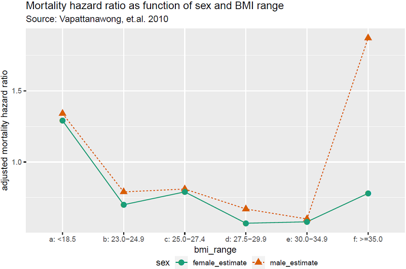
Figure 10.3. Example decision tree (from chapter 1)
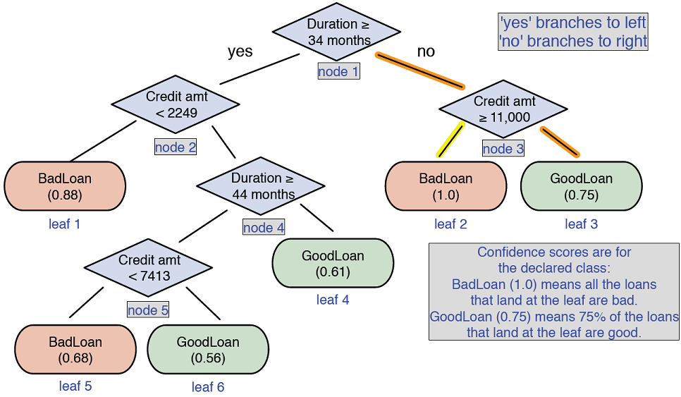
Figure 10.4. Decision tree model for spam filtering
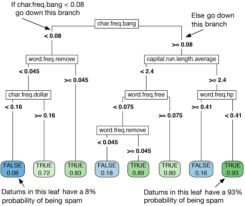
Figure 10.5. Bagging decision trees
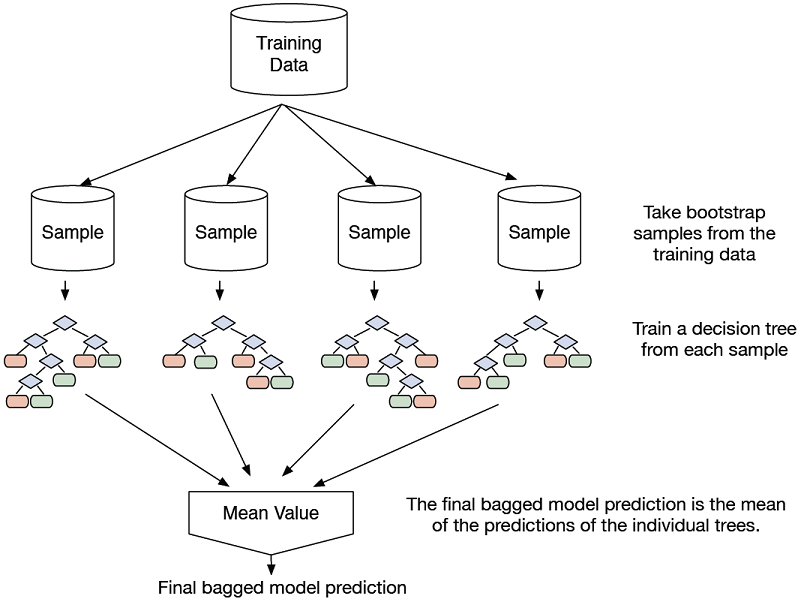
Figure 10.6. Growing a random forest
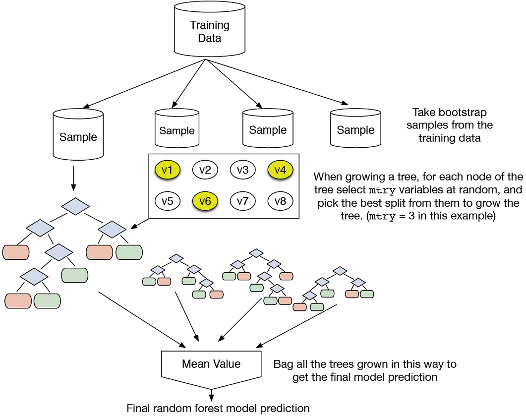
Figure 10.7. Out-of-bag samples for datum x1
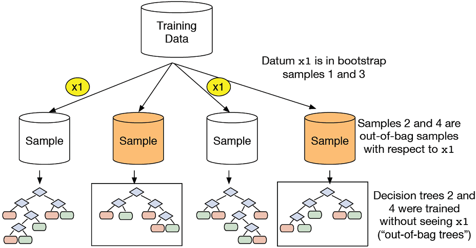
Figure 10.8. Calculating variable importance of variable v1
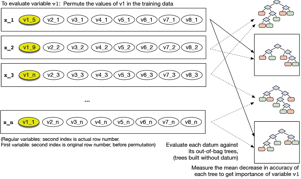
Figure 10.9. Plot of the most important variables in the spam model, as measured by accuracy
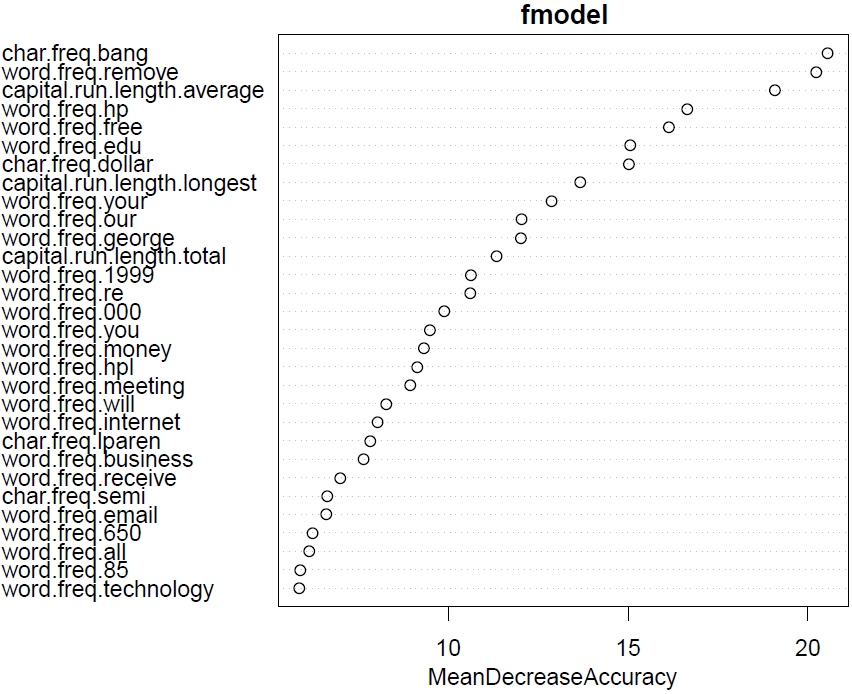
Figure 10.10. Building up a gradient-boosted tree model
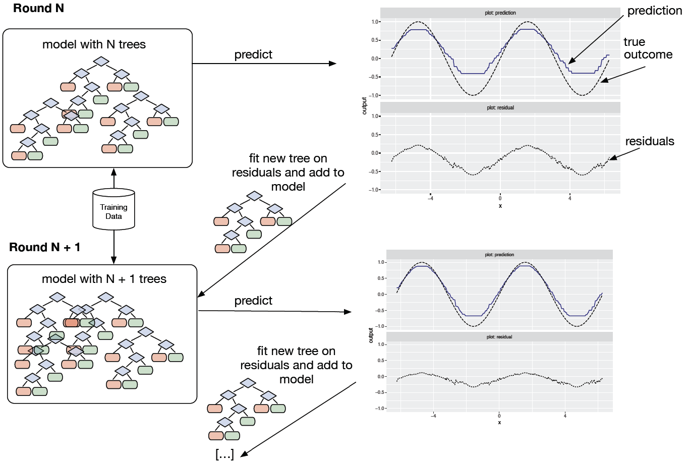
Figure 10.11. Cross-validated log loss as a function of ensemble size
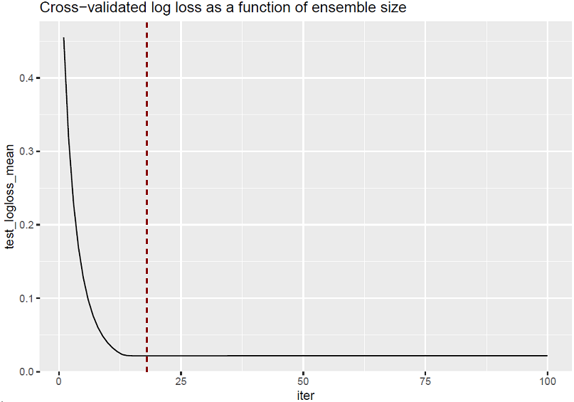
Figure 10.12. The effect of BMI on mortality: linear model vs. GAM
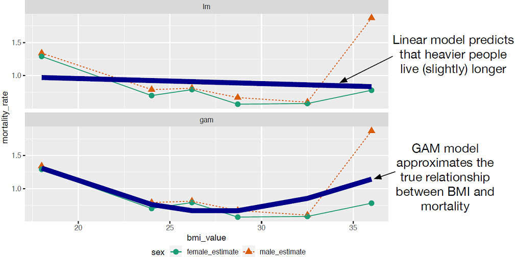
Figure 10.13. A spline that has been fit through a series of points
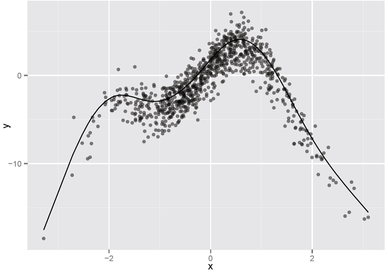
Figure 10.14. Linear model’s predictions versus actual response. The solid line is the line of perfect prediction (prediction == actual).

Figure 10.15. GAM’s predictions versus actual response. The solid line is the theoretical line of perfect prediction (prediction == actual).

Figure 10.16. Top: The non-linear function s(PWGT) discovered by gam(), as output by plot(gam_model) Bottom: The same spline superimposed over the training data

Figure 10.17. Smoothing curves of each of the four input variables plotted against birth weight, compared with the splines discovered by gam(). All curves have been shifted to be zero mean for comparison of shape.
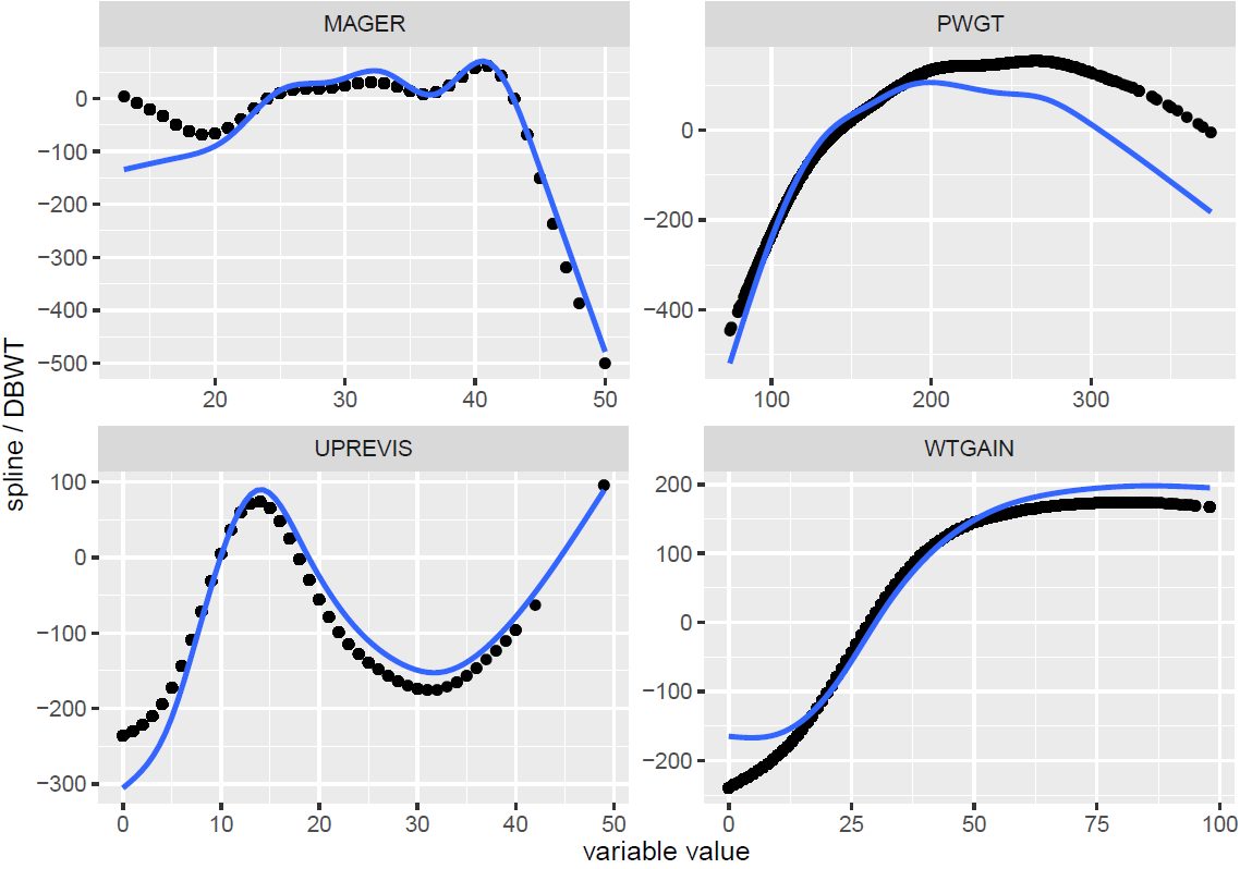
Figure 10.18. Notional illustration of a kernel transform (based on Cristianini and Shawe-Taylor, 2000)
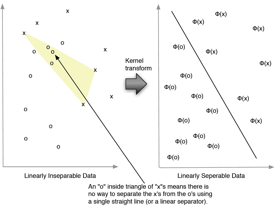
Figure 10.19. The spiral counter-example
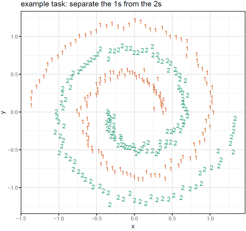
Figure 10.20. Identity kernel failing to learn the spiral concept
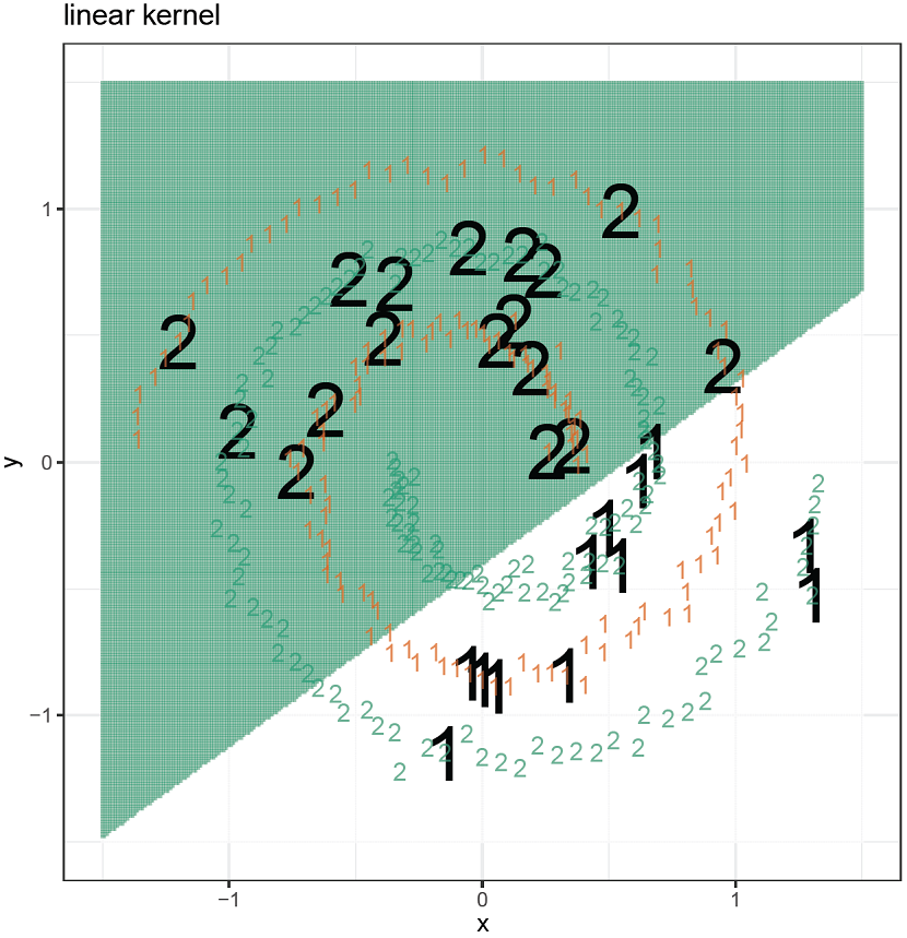
Figure 10.21. Radial kernel successfully learning the spiral concept
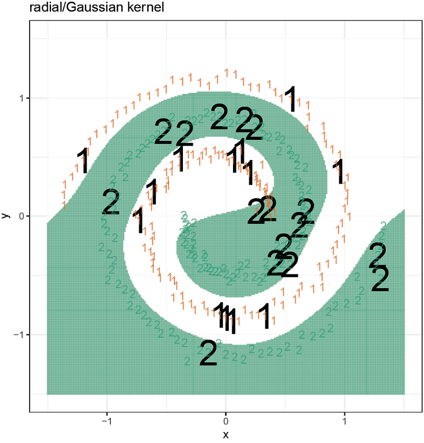
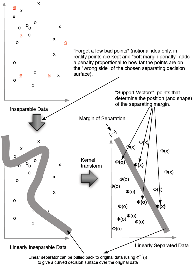
Figure 10.22. Notional illustration of SVM
Summary
In this chapter, we demonstrated some advanced methods to fix specific issues with basic modeling approaches: modeling variance, modeling bias, issues with non-linearity and with variable interactions. An important additional family of methods we wish we had time to touch on is deep learning, the improved modern treatment of neural nets. Fortunately there is already a good book we can recommend on this topic: Deep Learning with R, by François Chollet with J. J. Allaire, Manning 2018.
You should understand that you bring in advanced methods and techniques to fix specific modeling problems, not because they have exotic names or exciting histories. We also feel you should at least try to find an existing technique to fix a problem you suspect is hiding in your data before building your own custom technique; often the existing technique already incorporates a lot of tuning and wisdom. Which method is best depends on data, and there are many advanced methods to try. Advanced methods can help fix overfit, variable interactions, non-additive relations, and unbalanced distributions, but not lack of features or data.
Finally, the goal of learning the theory of advanced techniques is not to be able to recite the steps of the common implementations, but to know when the techniques apply and what trade-offs they represent. The data scientist needs to supply thought and judgement and realize that the platform can supply implementations.
In this chapter, you have learned:
- How to bag decision trees to stabilize their models and improve prediction performance.
- How to further improve decision-tree-based models by using random forests or gradient boosting.
- How to use random forest variable importances to help with variable selection.
- How to use generalized additive models to better model non-linear relationships between inputs and outputs in the context of linear and logistic regression.
- How to use support vector machines with the gaussian kernel to model classification tasks with complex decision surfaces, especially "nearest-neighbor" style tasks.
The actual point of a modeling project is to deliver results for deployment and to present useful documentation and evaluations to your partners. The next part of this book will address best practices for delivering your results.
FAQ
Why move beyond linear and logistic regression in Chapter 10?
Linear methods assume additive, monotone, and mostly linear relationships between inputs and outcome. Many real problems have non-linear effects and interactions (for example, U-shaped risks with BMI, or “if-then” combinations of variables). Chapter 10 introduces methods—tree ensembles, GAMs, and SVMs—that relax these assumptions and capture non-linearity and interactions.What are bagging, random forests, and gradient boosting, and how do they differ?
- Bagging: Fit many trees on bootstrap samples and average their predictions; reduces variance and stabilizes trees.- Random forests: Bagging plus random feature subsampling at each split (mtry) to de-correlate trees; typically stronger than plain bagging and offers OOB estimates and variable importance.
- Gradient boosting: Add trees sequentially to model residuals; very powerful but needs careful stopping/tuning to avoid overfitting.
How does bagging improve basic decision trees?
By training many trees on bootstrap-resampled datasets and averaging their outputs. This lowers model variance, improves accuracy and F1, and typically reduces overfitting versus a single tree. Classification should be based on averaged class probabilities (when available), not just majority vote of hard class labels.What makes random forests different from bagging, and how should I set mtry?
Random forests add feature randomness: at each split the algorithm samples a subset of features (mtry) before choosing the best split. This de-correlates trees and often improves test performance. Defaults in R’s randomForest are mtry ≈ p/3 for regression and ≈ √p for classification. If many features are informative, consider larger mtry; if not, smaller mtry speeds training.How does random forest variable importance work, and how can I use it?
Using out-of-bag (OOB) samples, the algorithm measures the drop in accuracy when a feature’s values are permuted. A larger average drop means higher importance. You can:- Identify key drivers and sanity-check model behavior.
- Reduce dimensionality (e.g., refit with top features) for smaller, faster models with similar accuracy.
What is gradient boosting and how do I control overfitting?
Gradient boosting adds trees one at a time to reduce residual errors from the current ensemble. It can overfit if you add too many trees or use overly complex trees. Mitigate by using cross-validation/early stopping, limiting tree depth, shrinking learning rate, and monitoring hold-out deviance/accuracy.How do I use xgboost with categorical or text data in R?
xgboost needs a numeric matrix. Options include:- For structured categoricals: use vtreat to produce numeric, NA-robust encodings. You can: (1) calibrate on a separate split with designTreatmentsN/…; (2) use mkCrossFrame… for cross-framed treatments; or (3) use designTreatmentsZ for a simpler one-step encode (similar to model.matrix but NA-robust).
- For text: build a document–term matrix (sparse) and pass it to xgboost.
What are generalized additive models (GAMs) and when should I use them?
GAMs fit an additive model where each predictor can have a smooth, non-linear effect s(x). They preserve interpretability like linear/logistic models while capturing non-monotone relationships. Use mgcv::gam() with s() terms; check effective degrees of freedom (edf): edf ≈ 1 suggests near-linear; larger edf indicates meaningful non-linearity. Validate on hold-out data to watch for overfit.How can I interpret and visualize GAM effects?
- Plot the smooths: plot(gam_model) shows each s(x).- Extract contributions: predict(gam_model, type = "terms") returns per-feature smooth contributions you can plot against the original variable.
- Compare to simple smooths of outcome vs. each feature to sanity-check shapes (bearing in mind GAM smooths are learned jointly).

 Practical Data Science with R, Second Edition ebook for free
