5 Simulated Annealing
This chapter introduces simulated annealing (SA) as a trajectory-based metaheuristic that navigates a search space with a single solution, occasionally accepting worse moves to escape local minima. Inspired by the physical annealing process, SA balances exploration and exploitation through a temperature-controlled stochastic search, contrasting with population-based methods that rely on multiple agents. The chapter positions SA as a general-purpose optimizer capable of handling continuous, discrete, and constraint satisfaction problems across design, planning, and control domains.
The core mechanics are framed through an energy analogy: solutions are states, the objective is energy, and temperature governs the probability of accepting non-improving moves via a Boltzmann-style rule. A concise pseudocode loop highlights initialization, neighborhood generation, probabilistic acceptance, and scheduled cooling. The chapter details cooling schedule design (initial/final temperature, iterations per temperature) and common schemes (linear, inverse-linear, geometric, logarithmic, exponential), then focuses on adaptivity—reheating, non-monotonic schedules, dynamically varying iterations, and modulating penalties in the objective—to improve robustness. It also summarizes practical trade-offs and variants (classical, fast, generalized, dual annealing), noting SA’s ease of use alongside parameter-tuning demands and occasionally slow convergence; quantum annealing is briefly contrasted conceptually.
Through case studies, the chapter shows SA solving continuous function optimization (from simple quadratics to multimodal benchmarks), discrete permutation problems like TSP, and constraint satisfaction such as Sudoku, plus a real-world delivery truck routing example. Results illustrate SA’s versatility: it reliably reaches global or near-optimal solutions on many continuous landscapes, delivers competitive TSP tours with suitable neighborhoods and initialization, and substantially improves real routing plans, though it does not guarantee optimality or feasibility. At the same time, structured problems with strong exact or specialized methods (e.g., hard Sudoku via backtracking or linear/integer programming) can outperform SA. The overarching guidance stresses careful temperature control, neighborhood design, adaptive strategies, and multiple runs to balance solution quality and computational cost.
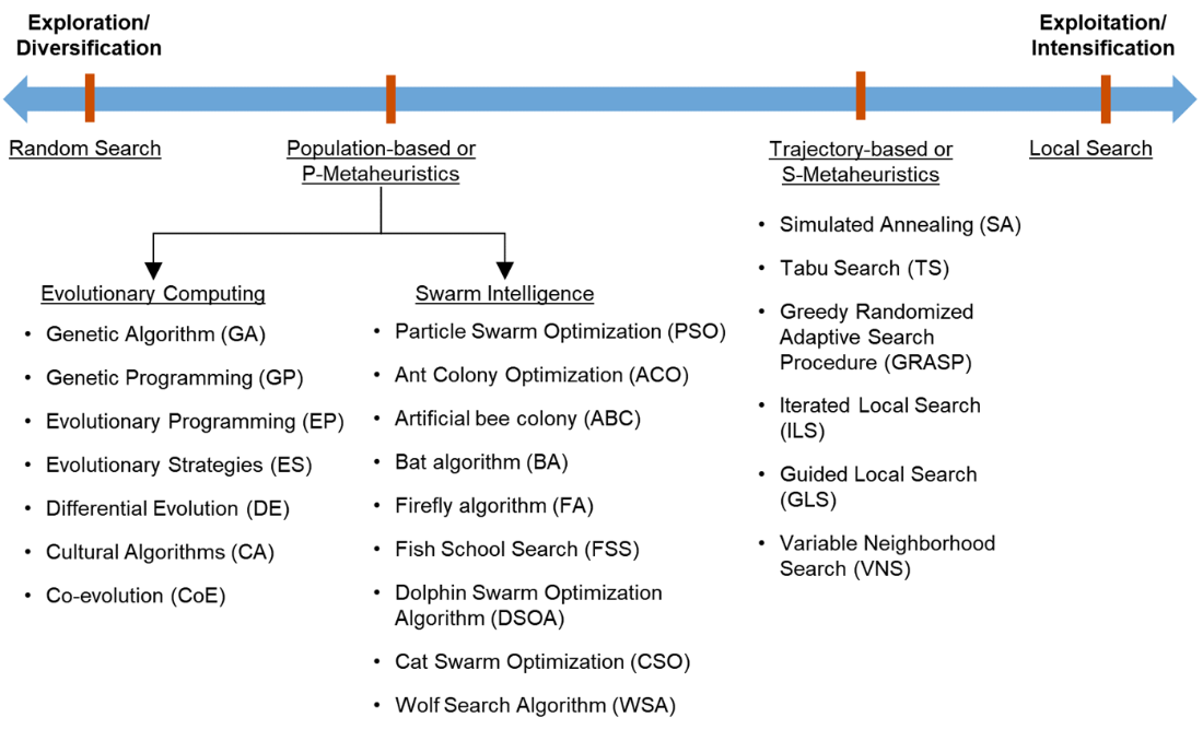
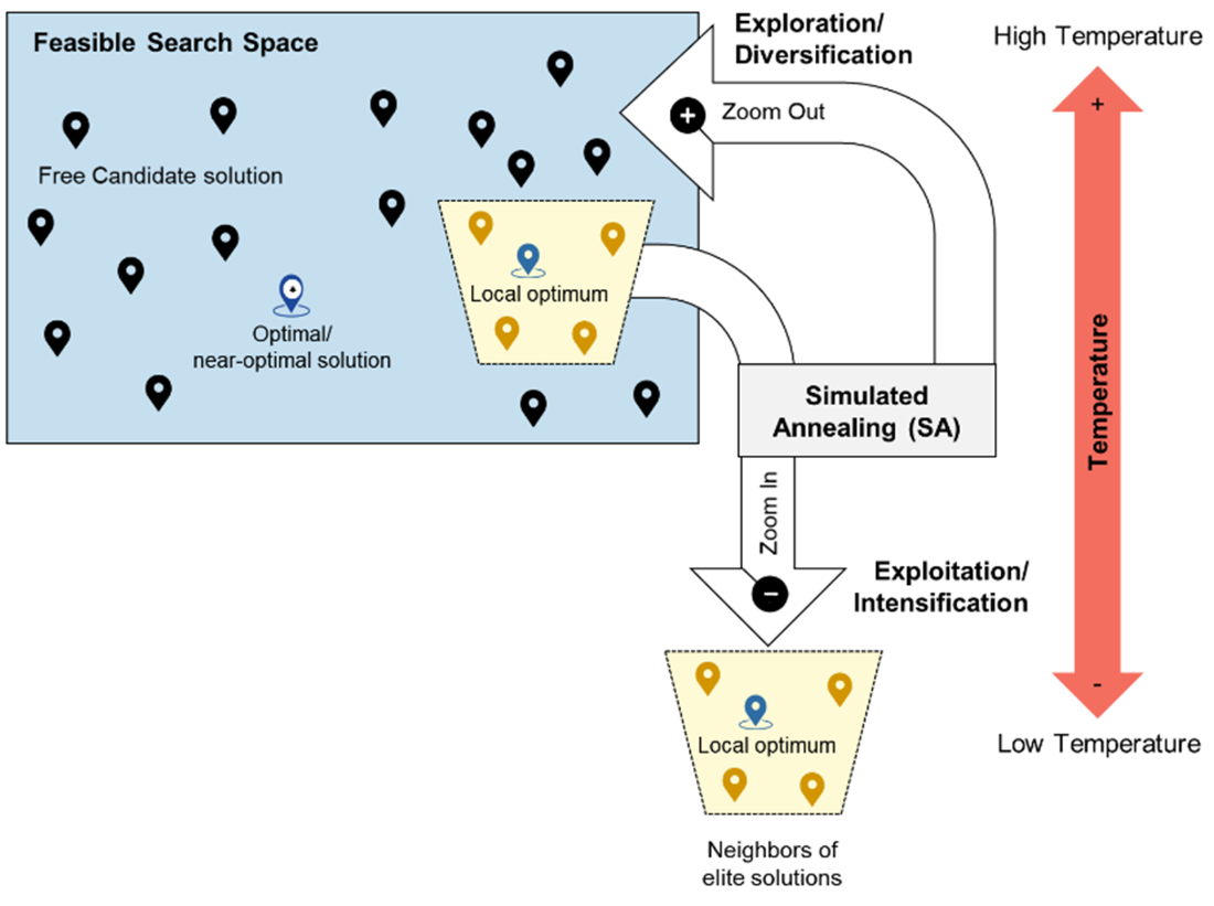
Exploration and exploitation of optimization algorithms
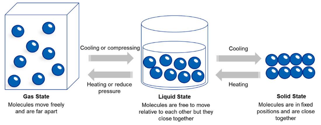
Effect of temperature on the mobility of the molecules.
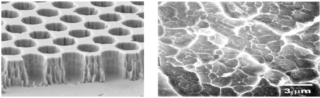
Physical annealing. Left: a metal with a crystalline structure. Right: Amorphous metal with a disordered atomic-scale structure.
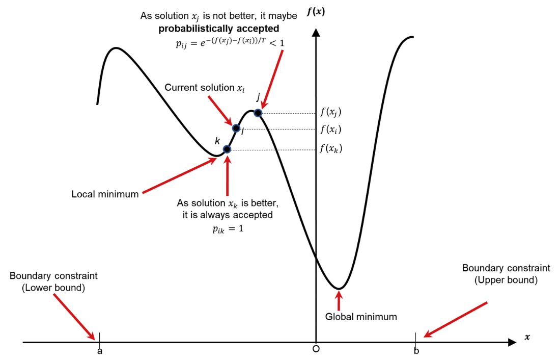
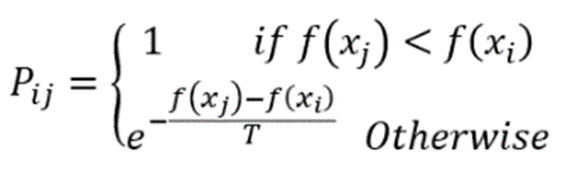
Transition probability. assuming a minimization problem, as solution 𝑥𝑘 is an improving move, it is always accepted and as solution 𝑥𝑗 is non-improving, it may be probabilistically accepted based on the transition probability.
Equation 5.4
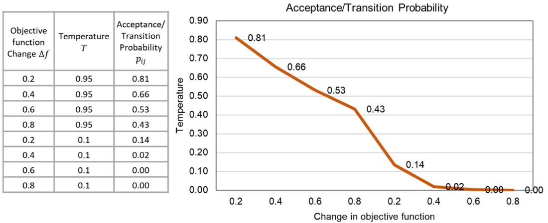
Change of acceptance probability with the temperature and the change in the objective function. At high temperatures, SA tends to explore more by accepting non-improving moves. As the temperature gets lower, the algorithm restricts exploration, favoring exploitation.
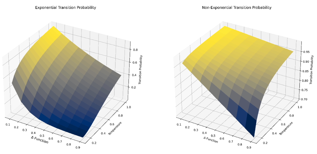
Exponential versus non-exponential transition probability.
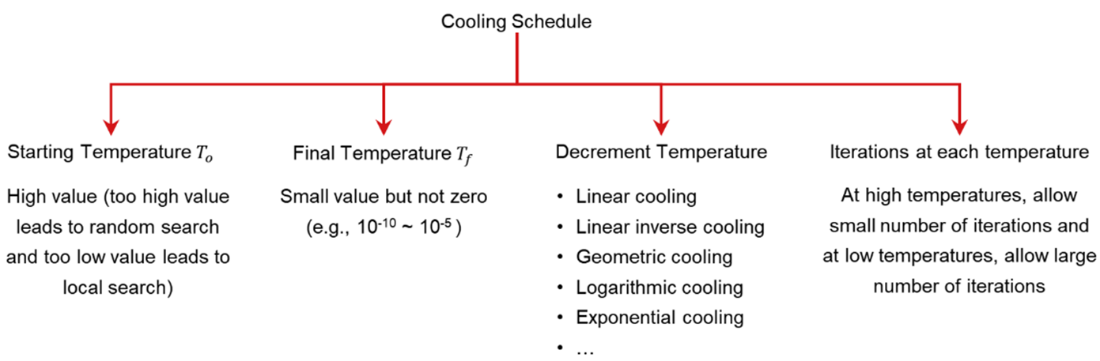
Cooling Schedule Components
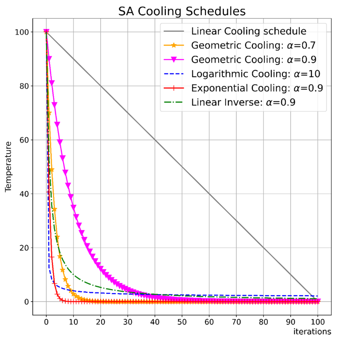
Different SA cooling schedules.
Effect of temperature. High temperatures result in more exploration and low temperature restricts the exploration and leads to more exploitation in the search space.
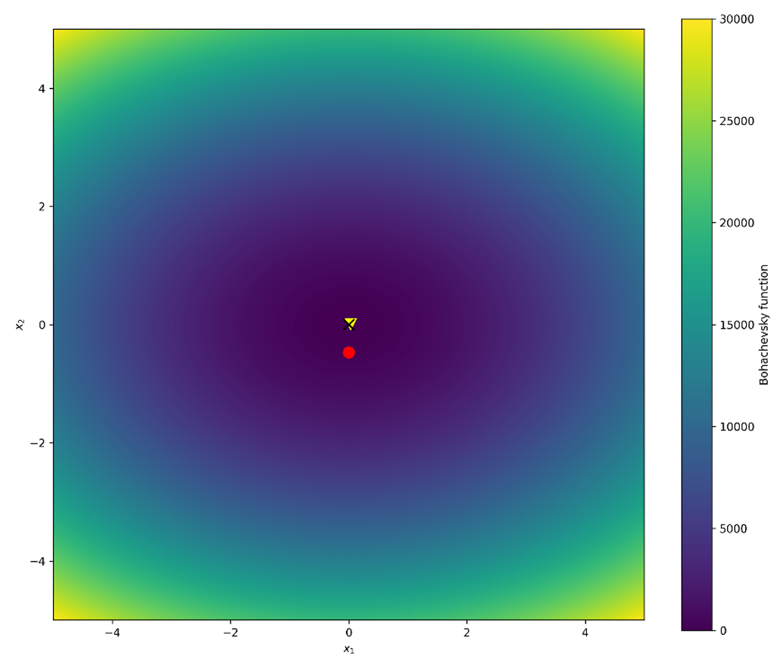
Solution of continuous function optimization problem using SA. Black cross is the optimal solution. Yellow triangle is the solution obtained by MEALPY SA. Red dot is the Scipy dual annealing solution.
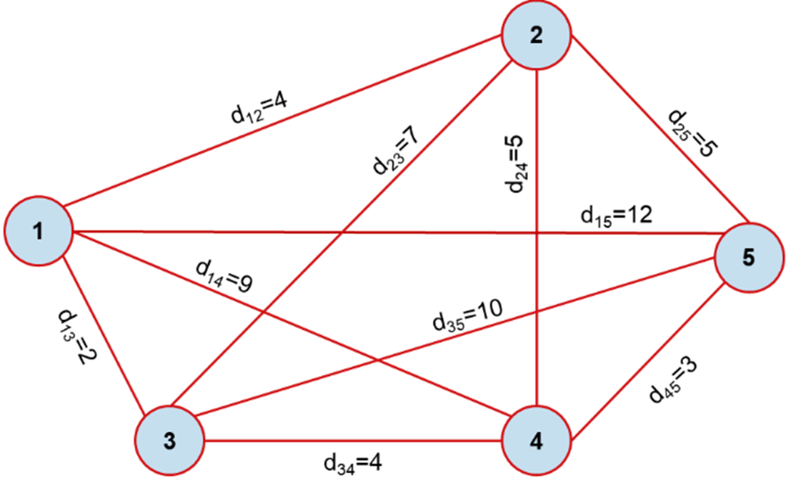
Travelling Salesman Problem (TSP) for 5 cities. There are 5!/2=60 possible tours assuming symmetric TSP.
SA Iteration-0 of 5-City TSP
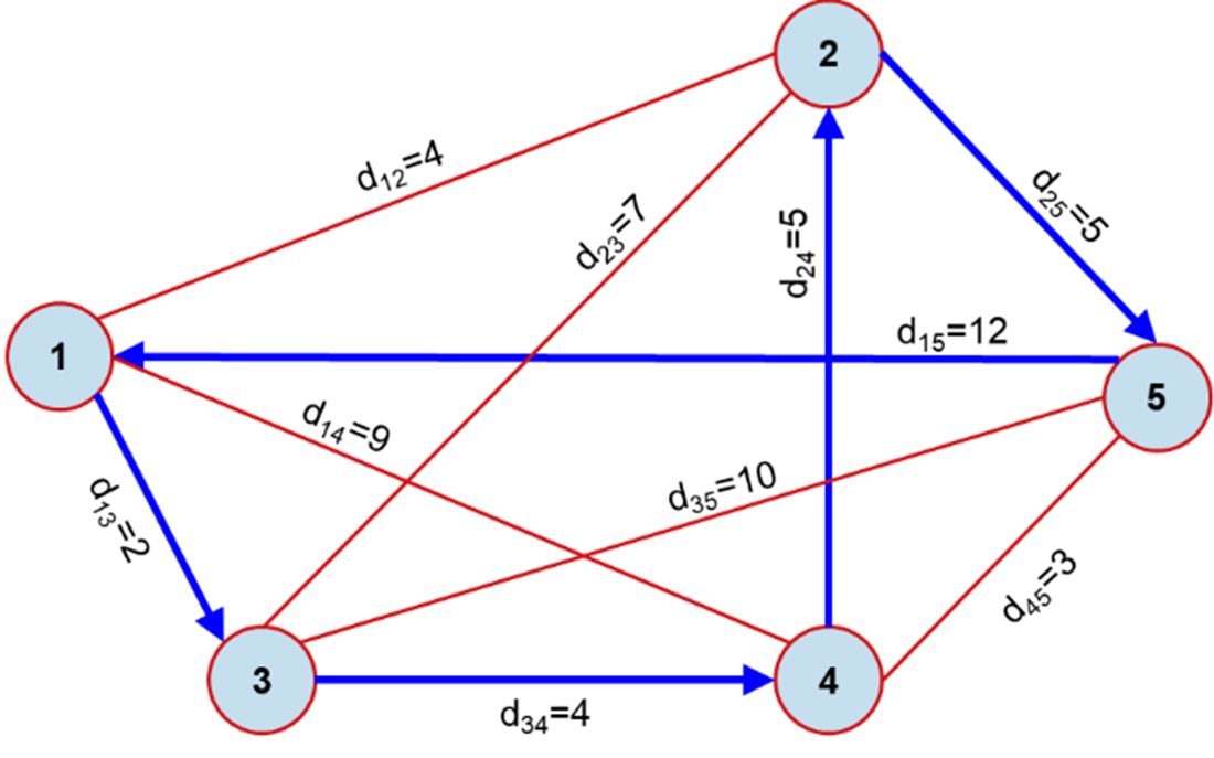
SA Iteration-1 of 5-City TSP
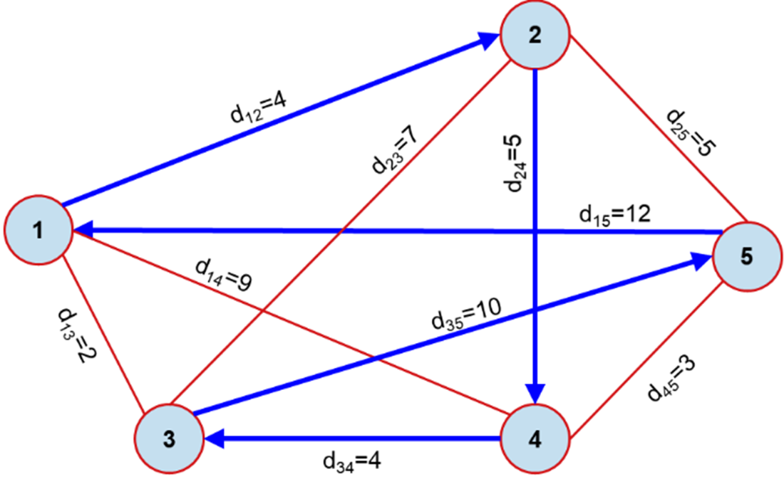
SA Iteration-2 of 5-City TSP
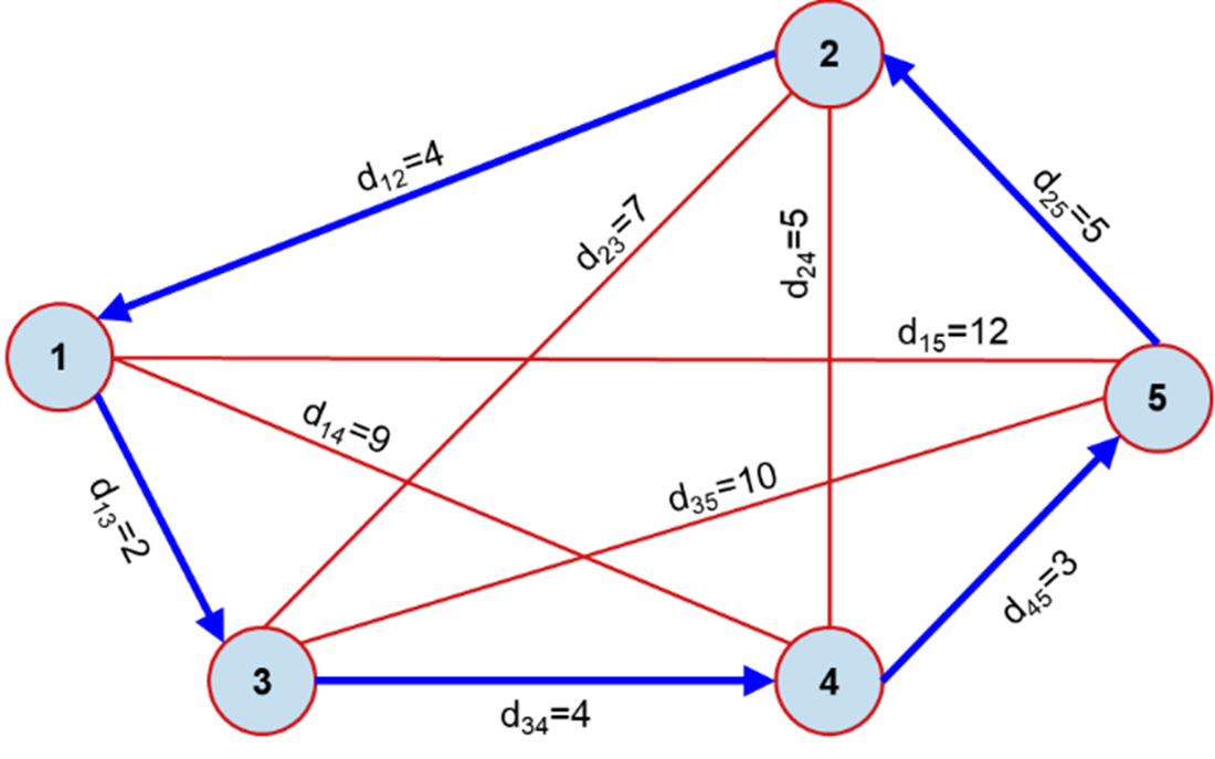
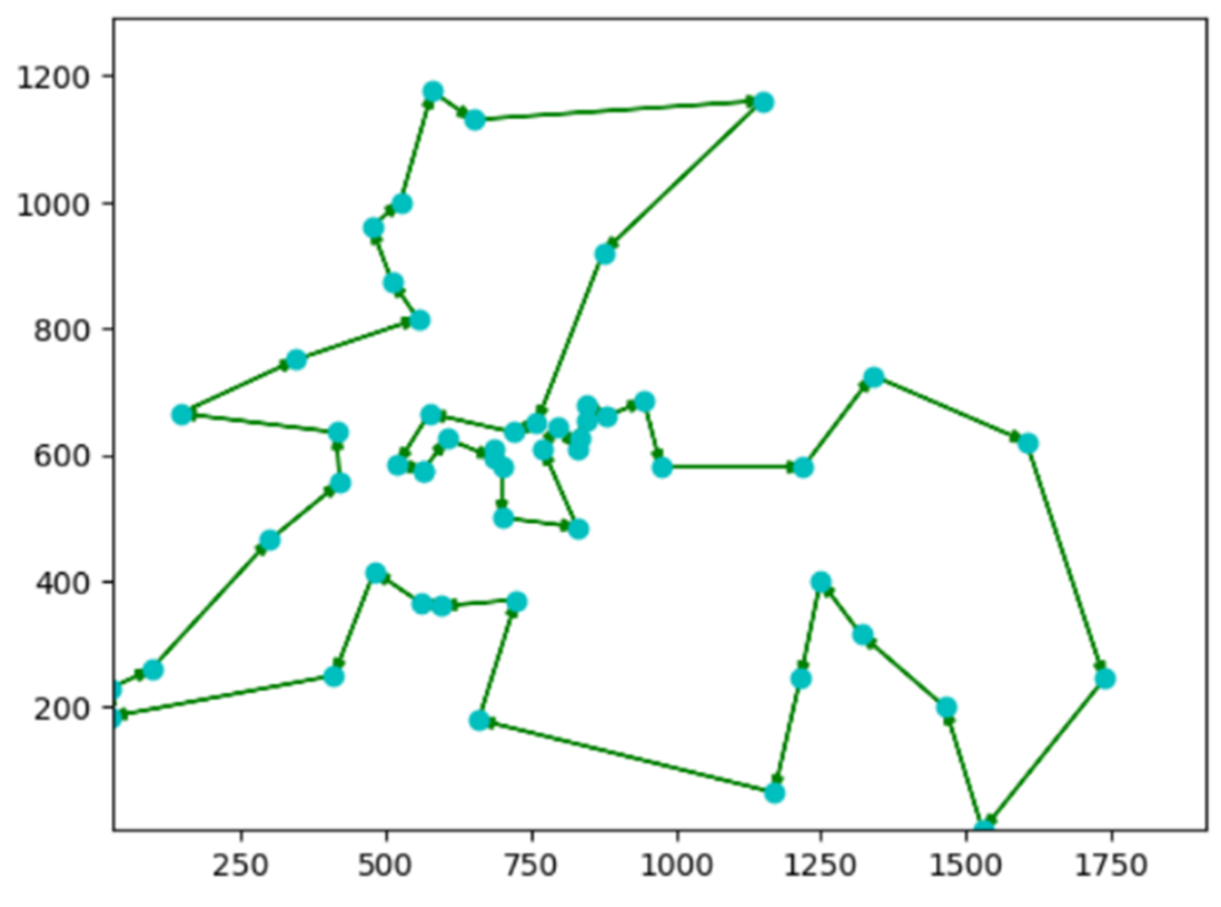
Solution of Belin52 using SA
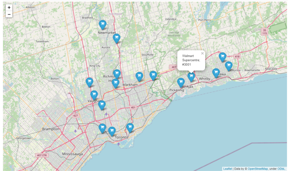
Selected Walmart Superstores in Greater Toronto Area (GTA).
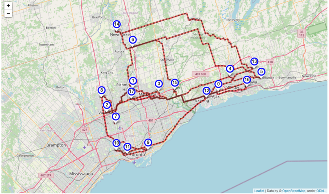
Initial Solution for Walmart delivery semi-truck route with total distance= 593.88 km
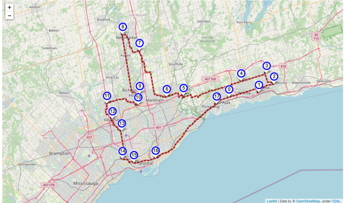
SA solution for Walmart delivery semi-truck route with total distance= 227.17 km
Summary
- Metaheuristic algorithms can be broadly classified into trajectory-based algorithms and Population-based algorithms. A trajectory-based metaheuristic algorithm or S-metaheuristics use a single agent or solution which moves through the design space or search space in a piecewise style. Population-based algorithms or P-metaheuristics use multiple agents to search for an optimal or near-optimal global solution. Simulated annealing is a trajectory-based metaheuristic algorithm.
- Simulated annealing mimics the annealing process in material processing when a metal cools and freezes into a crystalline state with the minimum energy and larger crystal size so as to reduce the defects in metallic structures. The annealing process involves the careful control of temperature and cooling rate, often called the annealing schedule.
- Simulated annealing runs a series of moves under different thermodynamic conditions and always accepts improving moves and can probabilistically accept non-improving moves.
- The acceptance probability is proportional to the temperature. High temperature increases the chance of accepting non-improving moves to favor exploration of the search space at the beginning of the search. As the search progresses, the temperature gets decremented to restrict exploration and favor exploitation.
- As the temperature goes to zero, SA acts greedily like hill climbing and as T goes to infinity, SA behaves like a random walk. The temperature should decrease gradually to achieve the best trade-off between exploration and exploitation.
- Simulated annealing is a stochastic search algorithm and a derivative-free solver that can be used when derivative information is unavailable, unreliable, or prohibitively expensive. SA seeks optimal or near-optimal solutions at a reasonable computational cost but it cannot guarantee either feasibility or degree of optimality.
- Adaptive simulated annealing can dynamically change its parameters with the search progress to control the exploration and exploitation behavior.
- Simulated annealing is an easy-to-implement probabilistic approximation algorithm that can be used to solve continuous and discrete problems in different domains.
FAQ
What is simulated annealing (SA) and why is it called “annealing”?
Simulated annealing is a trajectory-based metaheuristic that searches for a global optimum by occasionally accepting worse solutions to escape local minima. It is inspired by the physical annealing process where a material is heated and slowly cooled so its molecules settle into a low-energy (stable) crystalline state. In optimization, the “energy” maps to the objective (cost) value, and the controlled “cooling” of a temperature parameter guides the balance between exploration and exploitation.How is SA different from hill climbing and from population-based algorithms?
- Compared to hill climbing (greedy local search), SA may accept worse moves with a probability, helping it escape local minima; hill climbing accepts only improving moves.- SA is trajectory-based: a single solution moves through the search space step by step.
- Population-based methods (e.g., genetic algorithms, PSO, ACO) evolve multiple solutions simultaneously and naturally emphasize exploration due to population diversity.
How does SA decide whether to accept a worse move?
Let Δf be the change in the objective (minimization). If Δf ≤ 0, accept. If Δf > 0, accept with probability p = exp(−Δf / T), where T is the current temperature; equivalently, accept if exp(−Δf / T) > r for a random r ∈ [0, 1]. Alternatives to reduce computation include lookup tables or normalized non-exponential rules such as p(Δf) = 1 − Δf/T (clipped to [0, 1]).What does the temperature control, and what happens as it cools?
- High temperature: high acceptance of worse moves ⇒ strong exploration.- Low temperature: low acceptance of worse moves ⇒ strong exploitation (local refinement).
- At T → 0, SA reduces to hill climbing (no worse moves accepted). The cooling schedule determines how quickly the algorithm shifts from exploration to exploitation.
How should I choose the initial and final temperatures?
- Initial temperature (T₀): if max(Δf) is known, a practical estimate is T₀ ≈ −max(Δf) / ln(p₀) for a desired initial acceptance rate p₀ of worse moves. If unknown, start high and reduce until ~50–60% of worse moves are accepted; use that T as T₀.- Final temperature (T_f): often a small value (e.g., 1e−10 to 1e−5) or stop when the system is “frozen” (neither better nor worse moves get accepted). It’s usually unnecessary to reach exactly zero.
Which cooling schedules can I use, and what are their trade-offs?
- Linear: T = T₀ − β i, with β = (T₀ − T_f)/i_f; simple but needs an iteration budget and may cool too uniformly.- Linear-inverse: T(i) = T₀ / (1 + α i); cools faster early, slower later.
- Geometric: T(i) = T₀ α^i, 0 < α < 1 (commonly 0.7–0.95); smooth, widely used, no need to predefine max iterations in theory.
- Logarithmic: T(i) = T₀ / (1 + α log(1 + i)), α > 1; theoretical global convergence but often too slow in practice.
- Exponential: T(i) = T₀ exp(−α i^(1/n)); fast early cooling then slower, tunable by α and problem dimension n.
How many iterations should I run at each temperature?
Allow enough iterations per temperature to “stabilize” at that T. A common choice is a constant proportional to problem size (e.g., dimension for continuous problems or number of cities for TSP). Adaptive strategies work well: fewer iterations at high T (exploration), more at low T (exploitation) to thoroughly refine near local optima.How do I generate neighborhood solutions for continuous and discrete problems?
- Continuous: perturb variables with random noise, often Gaussian (normal) draws with chosen mean and standard deviation; clip to bounds as needed.- Discrete/permutation (e.g., TSP): use operators such as swap (random_swap), reverse (2-opt–like segment reversal), insert (remove and reinsert), or mutate (shuffle a block). For constraint problems, ensure feasibility or use penalties in the objective.
How can SA be adapted or enhanced in practice?
- Adaptive cooling: change schedule based on progress; e.g., reheating when stagnating or use T = (1 + (f_i − f*)/f_i) T(i) to react to current vs best objective.- Adaptive iterations per temperature: fewer at high T, more at low T.
- Adaptive penalties: gradually tighten constraint penalties over time.
- Variants: Fast SA (occasional long jumps), Generalized SA (Cauchy-Lorentz visiting distributions), Dual annealing (combines classical and fast SA with local search), and Adaptive SA (ASA) that auto-tunes temperature parameters.
- Quantum annealing (QA): uses quantum effects (tunneling) instead of thermal jumps to escape local minima; implemented on specialized hardware (e.g., D-Wave).
Where does SA work well, and what are its limitations?
- Strengths: simple, flexible, and effective for many continuous and discrete problems (e.g., nonlinear function optimization, TSP, routing). With tuning, it often finds near-optimal solutions and avoids many local minima.- Limitations: parameter tuning can be demanding; convergence can be slow; results vary run to run; feasibility and optimality are not guaranteed. For well-structured problems with strong deterministic solvers (e.g., 9×9 Sudoku), classical methods like backtracking or MILP can outperform SA in speed and reliability. For large TSPs (e.g., berlin52), SA may reach good but not best-known solutions without careful tuning or hybridization.

 Optimization Algorithms ebook for free
