12 Reinforcement Learning
This chapter introduces reinforcement learning (RL) as a framework in which agents learn by interacting with an environment to maximize cumulative reward. It lays out the core ingredients—states and observations, actions, policies (deterministic and stochastic), trajectories, returns, and value functions—and situates problems along a spectrum from Markov decision processes (MDPs), where actions affect future states, to multi-armed bandits (MABs), where state does not evolve. It also contrasts fully observable MDPs with partially observable settings, and outlines key learning paradigms: model-based vs model-free, and on-policy vs off-policy, motivating the exploration–exploitation trade-off as central to RL.
The chapter then surveys principal algorithms and architectures used in practice. It revisits dynamic programming ideas (value and policy iteration), moves to policy gradient methods, and explains advantage estimation as a stabilizing baseline. Actor–critic methods such as A2C split decision making (actor) from evaluation (critic), while Proximal Policy Optimization (PPO) controls policy updates either via a KL penalty or clipping to ensure stable improvement despite shifting data distributions. For bandit problems, it contrasts simple explore-only and exploit-only heuristics with ε-greedy and Upper Confidence Bound (UCB), using regret to quantify performance, and extends to contextual bandits that leverage side information to adapt action selection.
Finally, the chapter shows how RL can tackle real optimization and control tasks. It illustrates end-to-end pipelines and libraries (e.g., Stable-Baselines3 and RLlib) and demonstrates A2C/PPO on CartPole, centralized and multi-agent PPO for autonomous coordination in mobile networks, and contextual bandits (with Vowpal Wabbit) for combinatorial action selection in a truck assignment scenario. Beyond these worked examples, it highlights broader applications in routing (TSP/VRP), satisfiability and graph problems (MaxCut, MIS), ride-sharing, freight logistics, elevator dispatch, and traffic signal control—underscoring RL’s versatility for design, planning, and control under uncertainty.
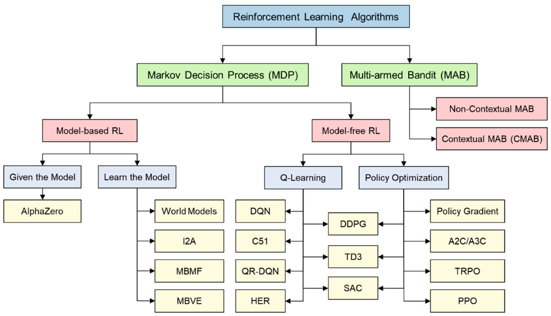
Reinforcement learning algorithm taxonomy
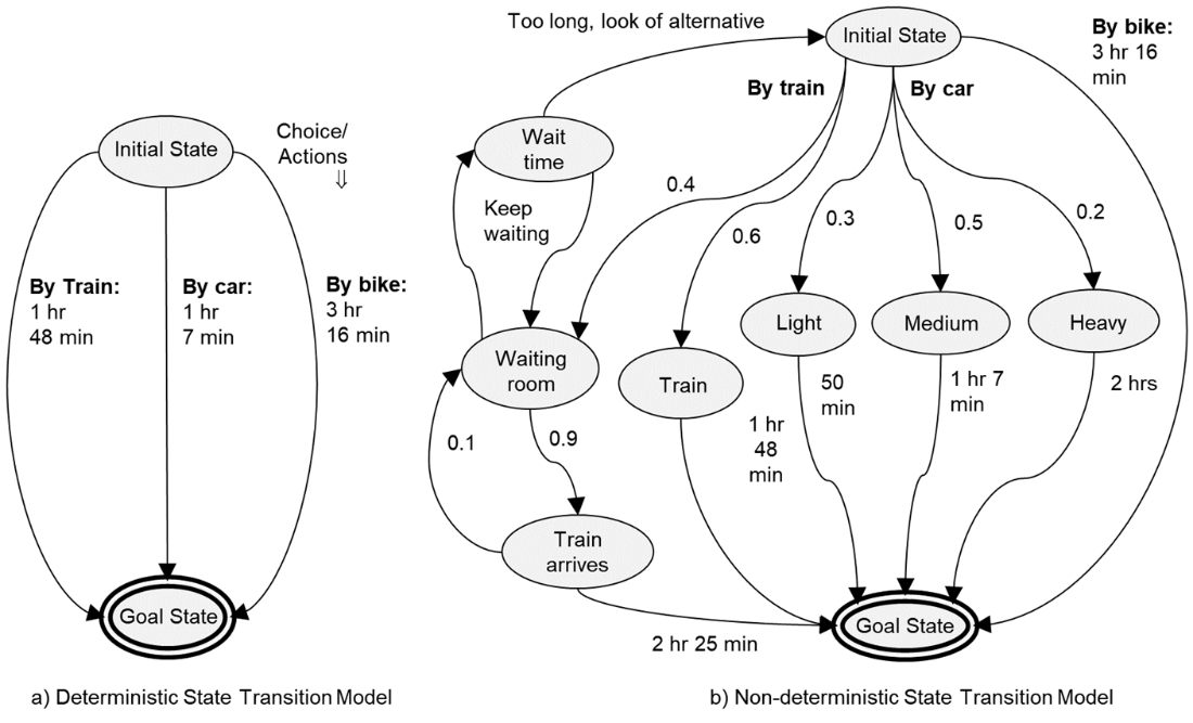
Deterministic versus non-deterministic state transition models
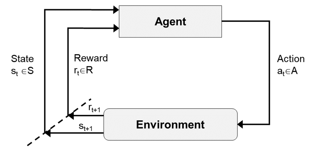
An agent learns through interaction with the environment
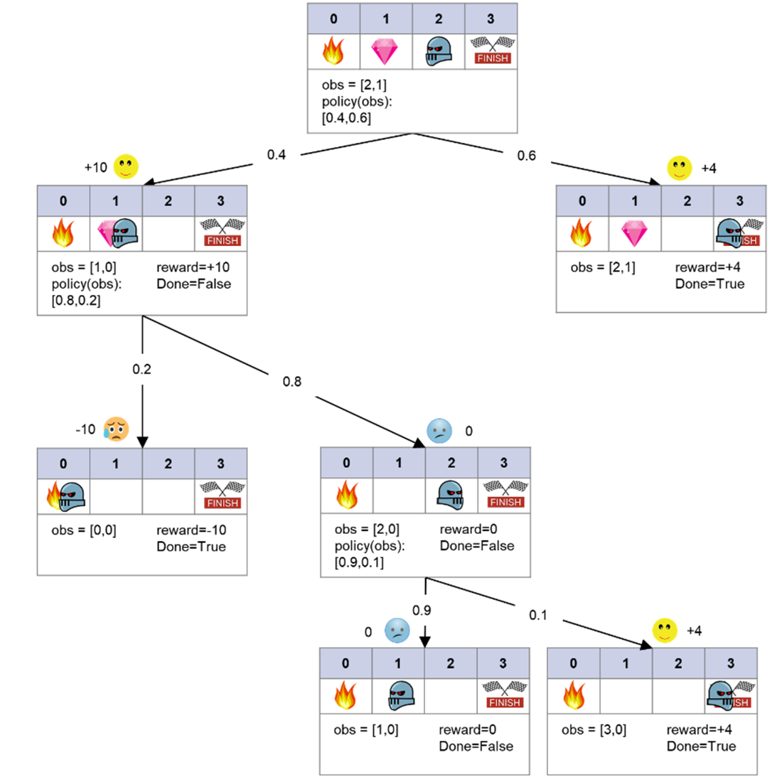
Reach a Treasure game
Equation 12.1
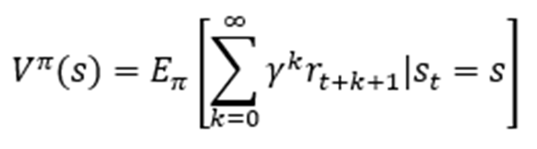
Equation 12.2
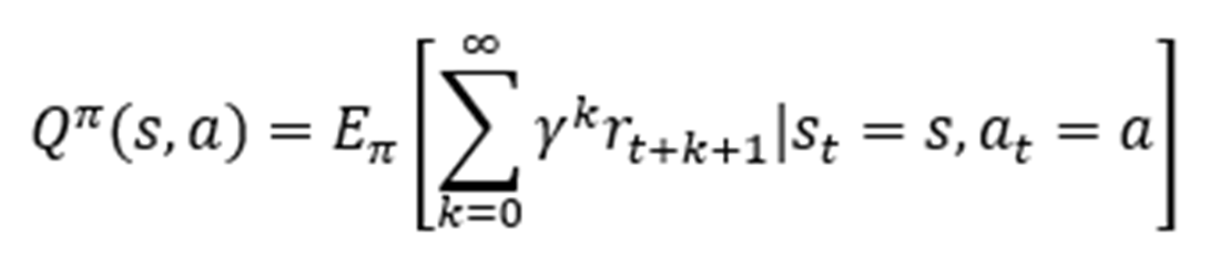
Equation 12.3

Equation 12.4

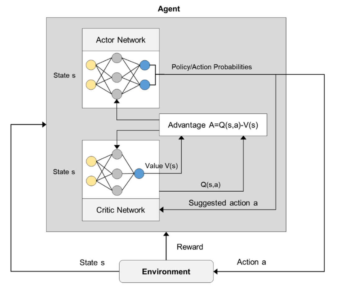
The Advantage Actor-Critic (A2C) Architecture
Equation 12.5
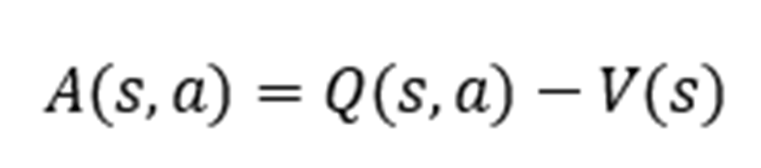
Equation 12.6

Equation 12.7

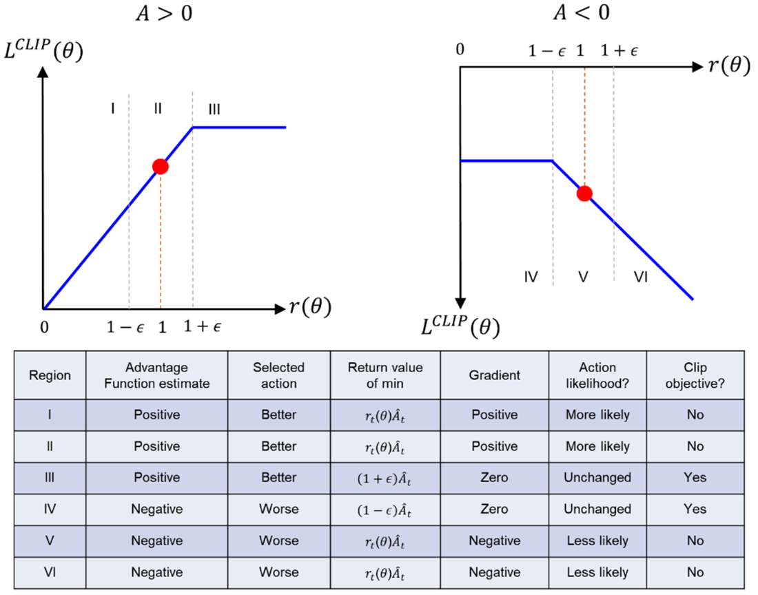
Clipped Surrogate Objective in PPO.
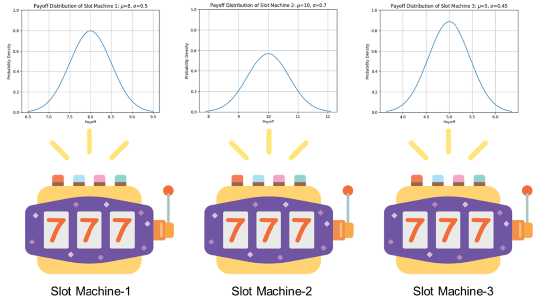
Three slot machines as non-contextual multi-armed (MAB) bandit problem. Payoff distribution’s mean and standard deviation of these three machines are (8,0.5), (10, 0.7) and (5, 0.45) respectively.
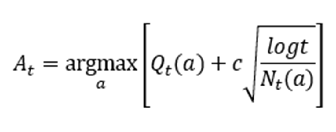
Equation 12.8
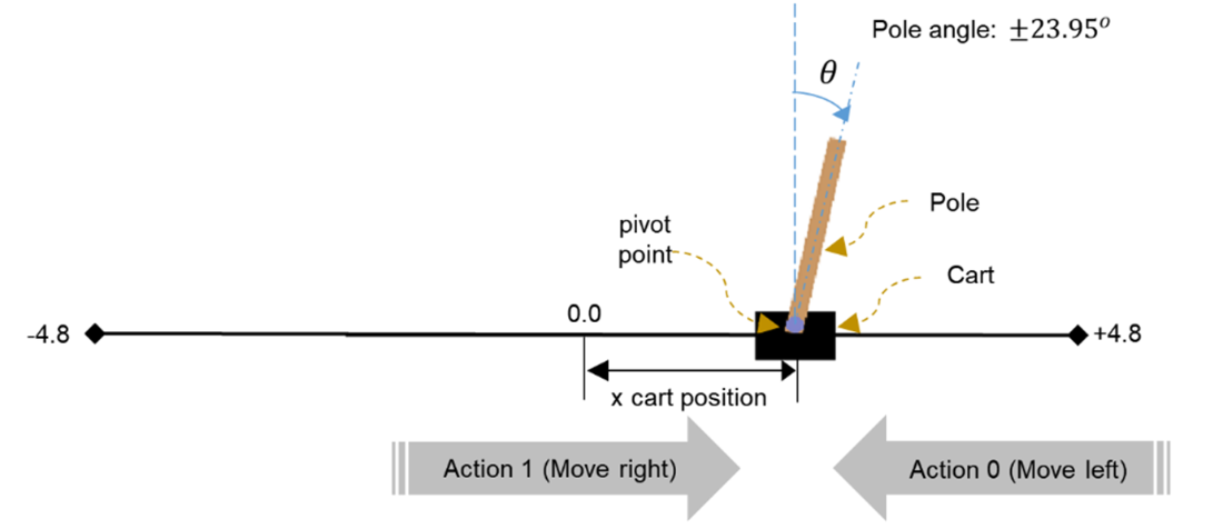
CartPole balancing problem
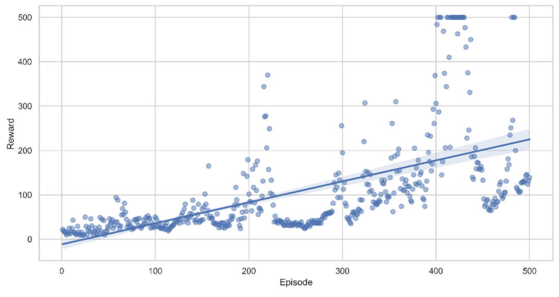
Episode rewards with the trend line
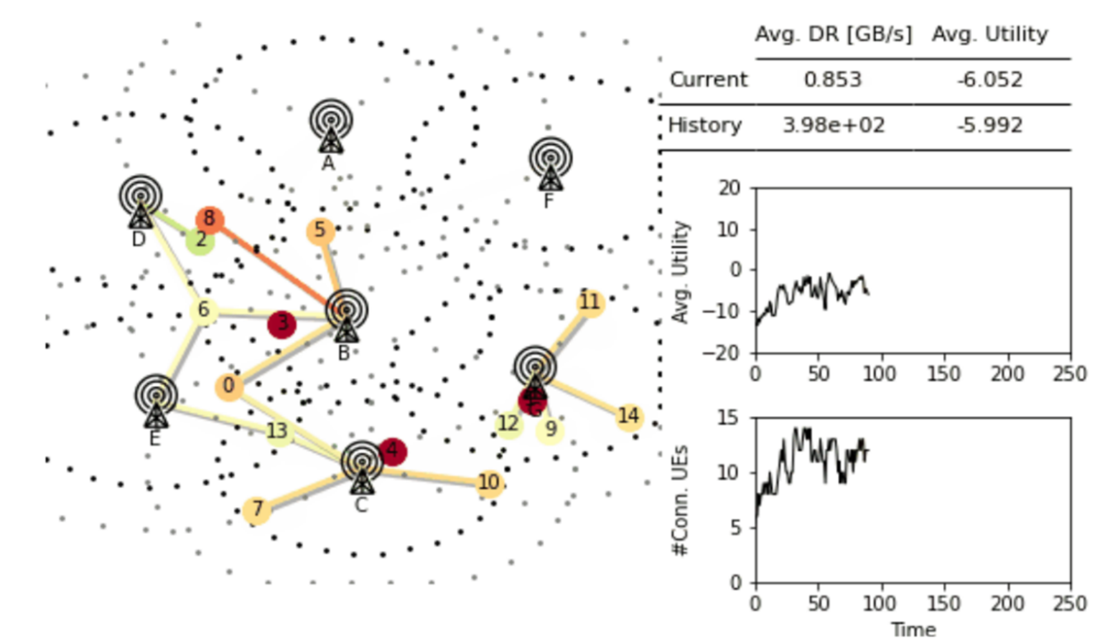
mobile-env: An Open Environment for Autonomous Coordination in Mobile Networks [13]
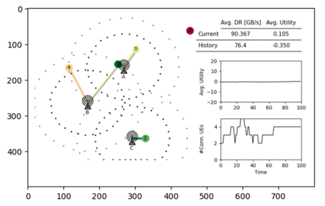
Coordination of mobile environment using multiagent PPO
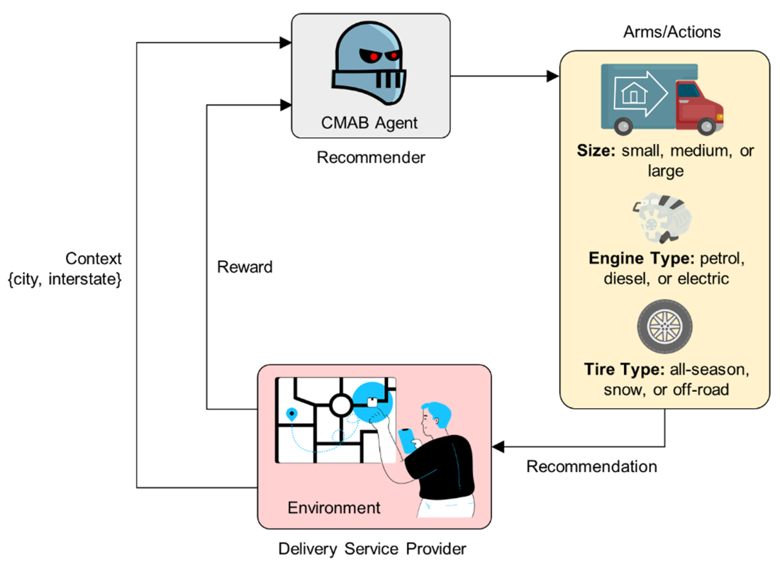
A CMAB-based recommender system to select delivery truck size, engine type and tire type based on a specified context.
Summary
- Reinforcement learning (RL) can be formulated as an optimization problem, wherein the agent aims to learn and/or refine its policy to maximize the expected cumulative reward within a specific environment.
- Reinforcement learning problems can be classified into Markov Decision Process (MDP) problems, where the agent's actions impact the environment and its future states, and Multi-Armed Bandit (MAB) problems, where the focus is on maximizing cumulative rewards from a series of independent choices (arms).
- In MDP-based problems, reinforcement learning uses MDP as a foundational mathematical framework to model decision-making problems under uncertainty. MDP is used to describe an environment for RL, where an agent learns to make decisions by performing actions in an environment to achieve a goal.
- RL is classified into model-based and model-free RL based on the presence or absence of a model of the environment. The model refers to an internal representation or understanding of how the environment behaves, specifically the transition dynamics and reward function.
- Based on how RL algorithms learn and update the policy from collected experiences, RL algorithms can be classified into off-policy and on-policy RL.
- A2C (Advantage Actor-Critic) and PPO (Proximal Policy Optimization) are model-free on-policy RL methods.
- By using a clipped objective function, PPO strikes a balance between encouraging exploration and maintaining stability during policy updates. The clipping operation restricts the update to a bounded range, preventing large policy changes that could be detrimental to performance. This mechanism ensures that the policy update remains within a reasonable and controlled distance from the previous policy, promoting smoother and more stable learning.
- Multi-armed bandit (MAB) is a reinforcement learning problem with a single state. ε-Greedy and Upper Confidence Bound (UCB) are examples of MAB strategies to determine the best approach for selecting the actions to maximize the cumulative reward over the time.
- Contextual Multi-Armed Bandits (CMAB) are an extension of MAB where the decision-making is influenced by additional contextual information about each choice or environment.
FAQ
What is Reinforcement Learning (RL) and how is it different from supervised learning?
RL is a learning paradigm where an agent interacts with an environment, takes actions, receives rewards or penalties, and aims to maximize expected cumulative discounted reward. Unlike supervised learning, RL does not rely on a fixed labeled dataset; the data distribution depends on the current policy, and exploration-exploitation trade-offs are central to learning.What is a Markov Decision Process (MDP) and when should I use a POMDP instead?
An MDP models decision-making under uncertainty with states, actions, transition probabilities, rewards, and a discount factor. It assumes full observability: the current state and action define the next-state distribution. If the agent only has partial observations of the true state, the problem is modeled as a POMDP.How do MDPs differ from Multi-Armed Bandits (MAB) and Contextual Bandits (CMAB)?
- MDPs: sequential decisions with state transitions; actions affect future states.- MABs: single-state problems; the agent repeatedly chooses among “arms” to maximize reward; no state transitions.
- CMABs: like MABs but with context (side information) that influences which arm is best at each step.
What are policy, value functions, Q-values, advantage, and discount factor in RL?
- Policy (μ or π, often πθ): mapping from states/observations to actions; can be deterministic or stochastic/parameterized.- Return: cumulative (possibly discounted) sum of future rewards.
- V(s): expected return from state s under a policy.
- Q(s,a): expected return from taking action a in state s under a policy.
- Advantage A(s,a): relative benefit of action a in s, typically A = Q − V.
- Discount γ: weights near-term rewards more than distant ones (0 ≤ γ < 1).
What’s the difference between model-based and model-free RL?
- Model-based: learns or uses a model of environment dynamics and rewards to plan; can be sample-efficient but requires accurate models (e.g., Expert Iteration, I2A).- Model-free: learns value/policy directly from experience without explicit dynamics (e.g., Q-Learning, A2C/A3C, PPO); simpler but often less sample-efficient.
How do on-policy and off-policy methods compare?
- On-policy (e.g., REINFORCE, A2C, PPO): learn from data generated by the current policy; simpler, but less sample-efficient since past data is typically discarded after updates.- Off-policy (e.g., Q-Learning, DDPG, TD3, SAC): learn from data generated by a different behavior policy or replay buffer; more sample-efficient but require off-policy corrections.
What are actor-critic methods and what role does A2C play?
Actor-critic methods train two networks: the actor (policy) proposes actions and the critic (value function) evaluates them. A2C (Advantage Actor-Critic) synchronously updates both, using the advantage estimate to stabilize policy updates and improve sample efficiency.What problem does PPO solve and how do PPO-Clip and PPO-Penalty differ?
Policy gradients can make overly large updates on non-stationary data, destabilizing training. PPO constrains updates to stay “close” to the old policy:- PPO-Penalty: adds a KL divergence penalty to discourage big policy changes.
- PPO-Clip: uses a clipped surrogate objective on the probability ratio r(θ), limiting updates when they would push r outside [1−ε, 1+ε].
How is exploration-exploitation handled in bandits, and what is regret?
Bandits balance exploring uncertain arms and exploiting known good ones. Common strategies include:- Explore-only and Exploit-only (extremes, usually suboptimal).
- ε-Greedy: explore with probability ε, otherwise exploit the best estimated arm.
- UCB: choose actions using an optimism-in-the-face-of-uncertainty bonus. Regret measures the performance gap versus always playing the optimal arm.
How does the chapter apply RL to real problems like control and optimization?
- CartPole control: learn to balance a pole using A2C or PPO (from scratch or via Stable-Baselines3).- Mobile networks: PPO learns cell selection/coordination to maximize QoE; also shown in a multi-agent PPO setup (Ray RLlib).
- Contextual optimization: a CMAB example (truck selection) uses Vowpal Wabbit to choose size/engine/tire given route context to maximize expected utility.
- Broader optimization links include TSP/VRP, traffic signal control, and dispatch problems.

 Optimization Algorithms ebook for free
