Overview

Appendix C. Exercises and Solutions

This appendix gathers a comprehensive, chapter-aligned set of exercises with full solutions designed to bridge theory and practice across the book’s topics. It blends MCQs, true/false, short-answer reasoning, modeling and classification tasks, and hands‑on coding assignments. The material reinforces fundamentals (e.g., computational complexity, problem types, and modeling choices) while steadily moving into algorithmic design, performance trade‑offs, and practical implementation details, encouraging readers to verify concepts, compare strategies, and iteratively improve solutions.

The scope is broad and application‑oriented. Early sections revisit blind and informed search (BFS/DFS, UCS, A*, best‑first, hill climbing, contraction hierarchies), complexity classes (P, NP, co‑NP, NP‑hard/complete), and optimization modeling (decision variable structure, objective types, hard/soft constraints, LP/QP/NLP). Subsequent chapters dive into metaheuristics—simulated annealing, tabu search, genetic algorithms and variants, particle swarm optimization, and ant colony optimization—then expand to supervised/unsupervised learning (SOMs, attention, graph learning) and reinforcement learning (bandits, A2C/PPO, vectorized training). The exercises repeatedly ground ideas in real‑world contexts: routing and trip planning, facility location and districting, feed‑mix and knapsack‑like loading, composite laminates, open‑pit mining, school transport, ridesharing, trilateration, and resource allocation.

Solutions are implementation‑centric, with step‑by‑step Python examples and reproducible workflows. They employ widely used libraries and toolkits—PuLP for LPs, NetworkX and OSMnx for routing, simanneal and custom SA, optalgotools for TS and TSP, pymoo for GA/NSGA‑II, pyswarms for PSO, Stable‑Baselines3 for RL (A2C/PPO), Vowpal Wabbit for contextual bandits, and MIDACO and GEM for specialized ACO and motor‑control settings. Classic benchmarks (Rosenbrock, Ackley, Schwefel, TSP) sit alongside domain cases (e.g., feed‑mix LP, school bus scheduling, cargo bike loading, airliner service design). Throughout, the appendix emphasizes data handling, parameter tuning, visualization, and head‑to‑head method comparisons (e.g., cooling schedules in SA, operator choices in GA, node ordering in CH), equipping readers to experiment, evaluate, and generalize solutions beyond the given instances.

Figure C.1 Each item has a utility and a weight, and we want to maximize the utility of the contents of the knapsack. The problem is constrained by the capacity of the bag.
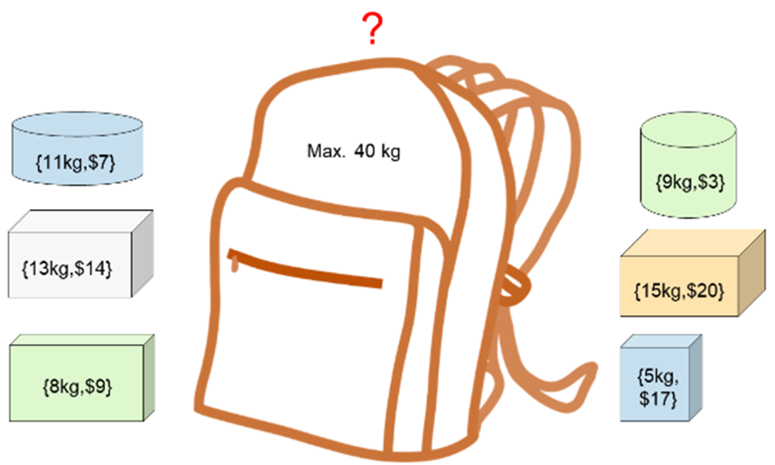
Figure C.2 Simplified map.
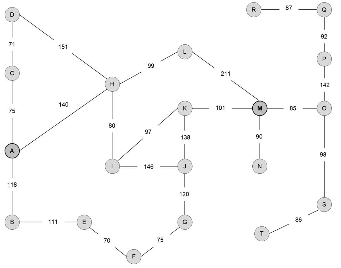
Figure C.3 A graph search exercise
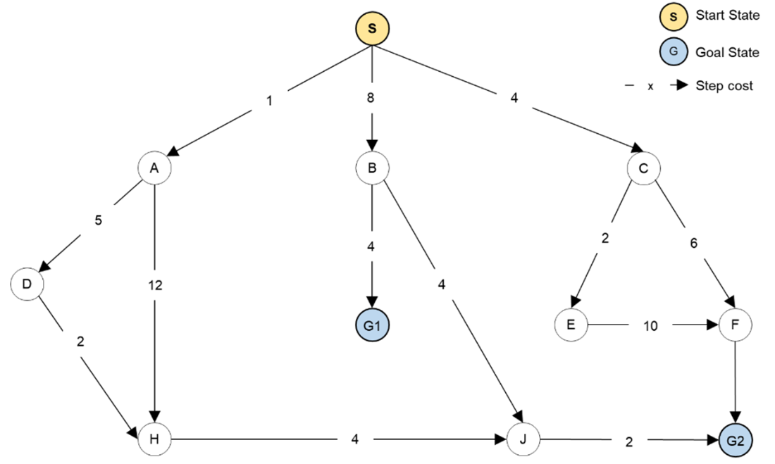
Figure C.4 Blind search crossword puzzle
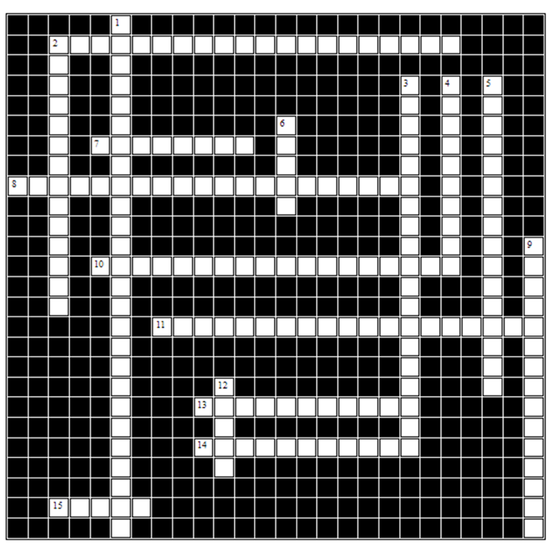
Figure C.5 Blind search crossword puzzle solution
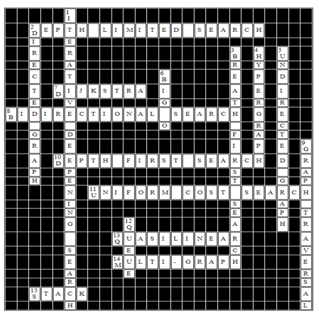
Figure C.6 Contracting node E
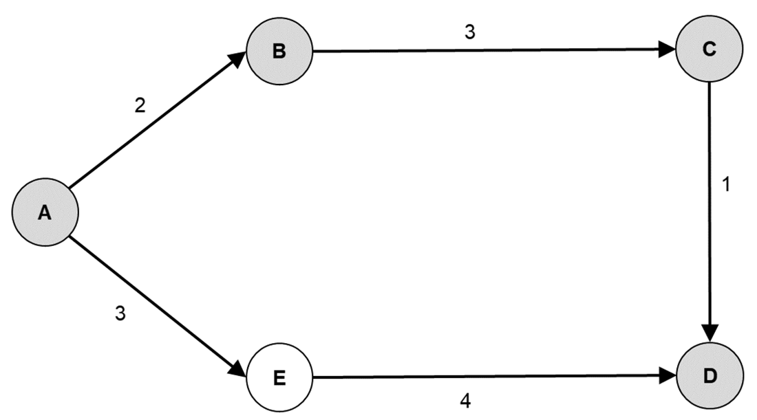
Figure C.7 Directed graph
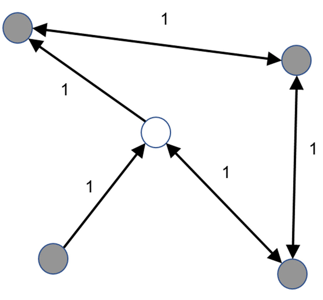
Figure C.8 Search space
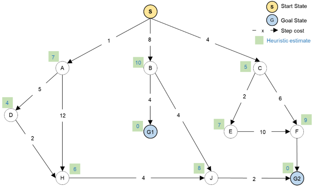
Figure C.9 Informed search word search puzzle
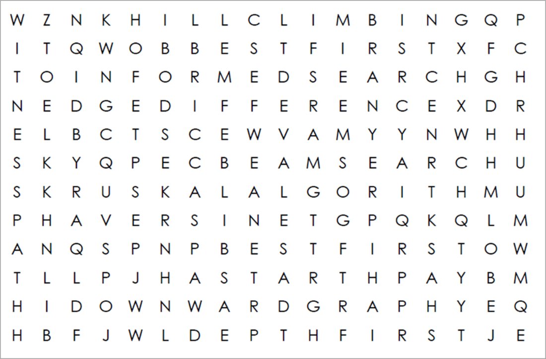
Figure C.10 Informed search word search puzzle solution
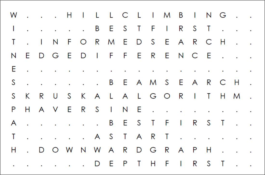
Figure C.11 Travelling Salesman Problem (TSP) for 20 largest US cities.
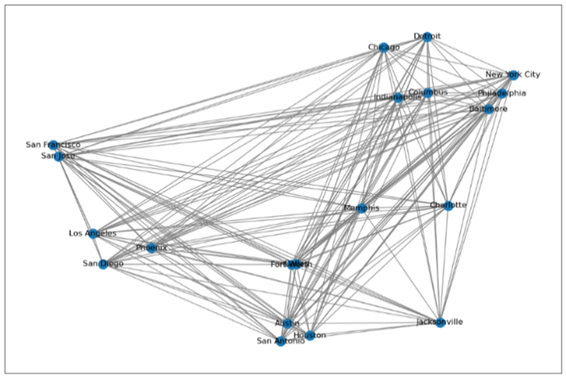
Figure C.12 Simulated annealing crossword puzzle
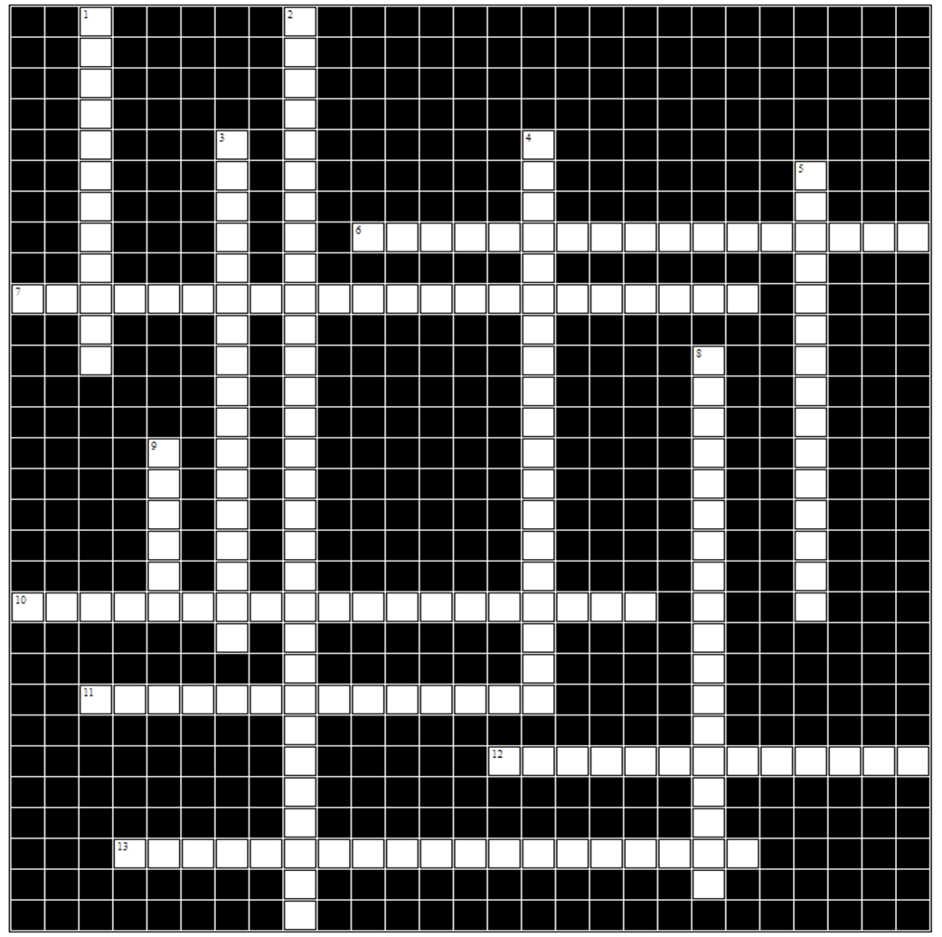
Figure C.13 Solution of 20 largest US cities TSP using simanneal
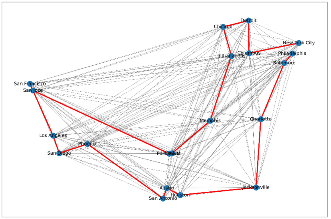
Figure C.14 Simulated annealing crossword puzzle solution
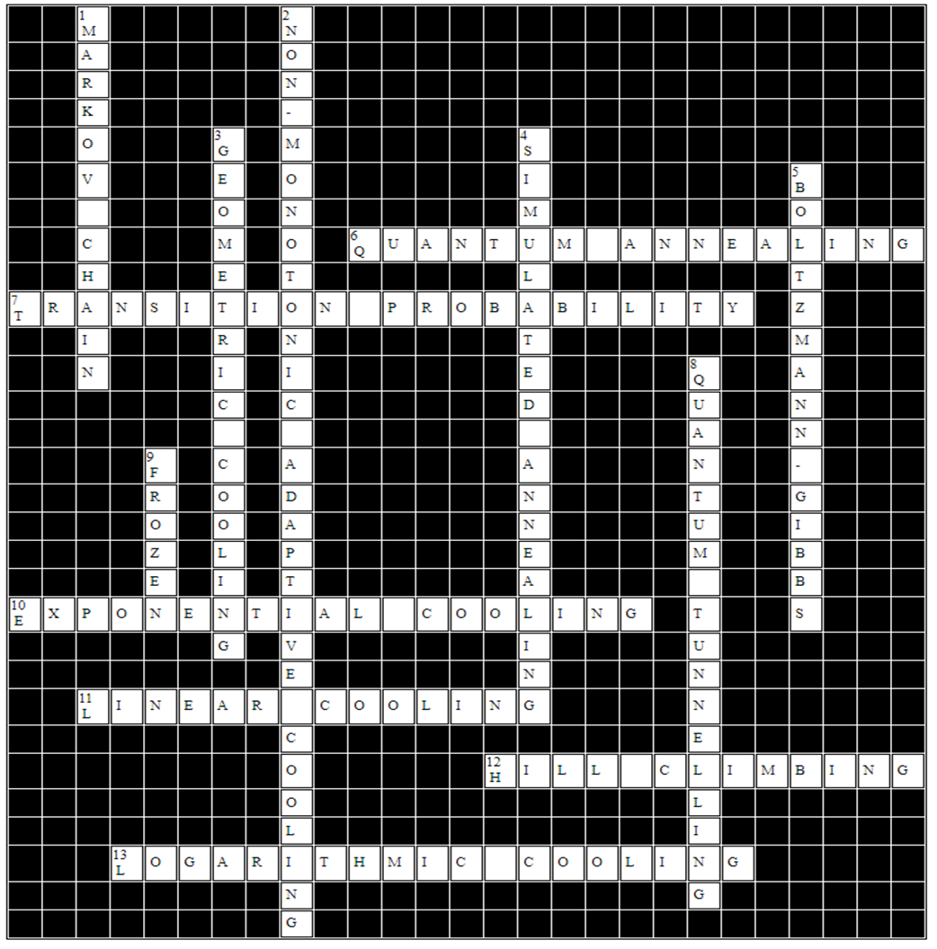
Figure C.15 Schwefel function
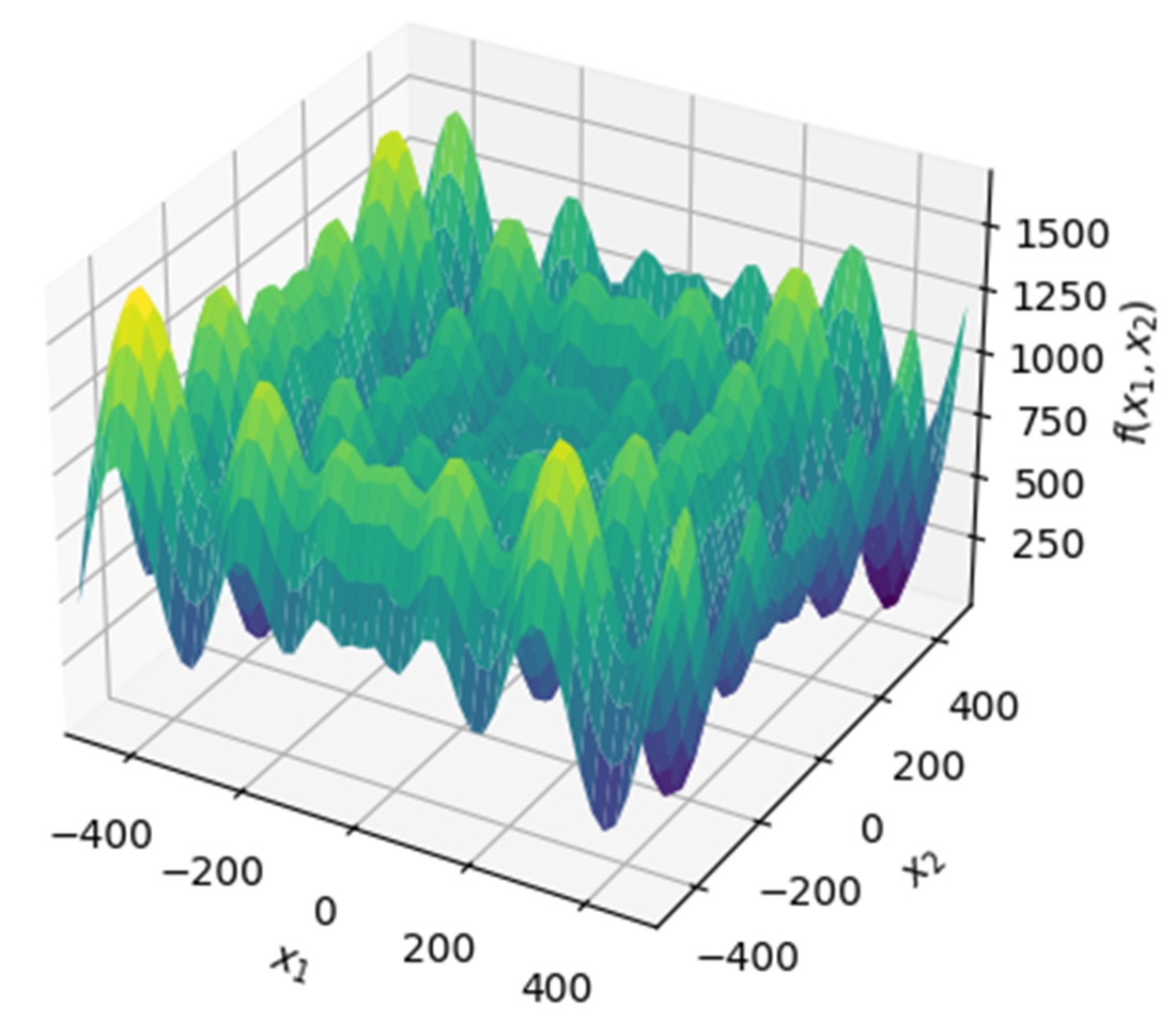
Figure C.16 Composite Laminate Design - Apple’s US Patent 7790637 B2
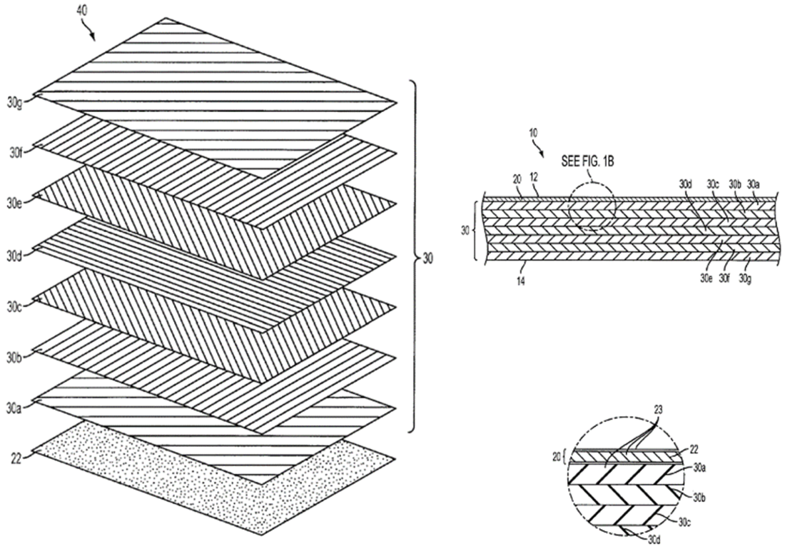
Figure C.17 Pairwise strength gain/loss
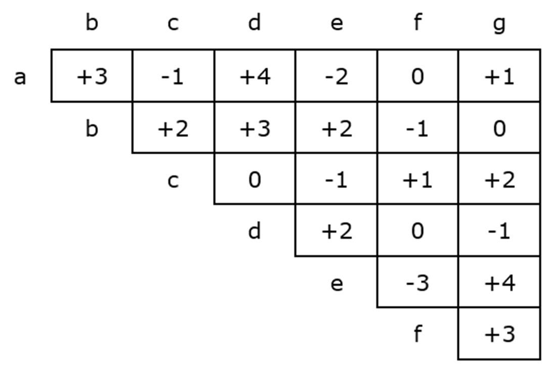
Figure C.18 TS word search puzzle
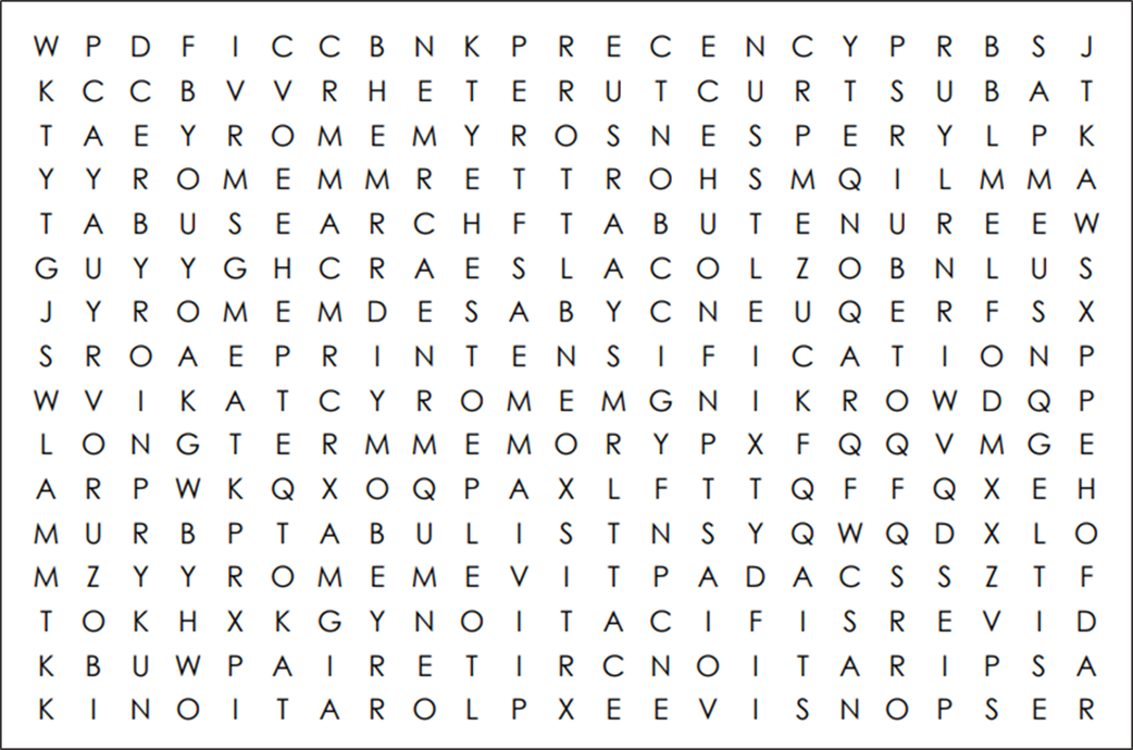
Figure C.19 Composite Laminate Design - TS Initialization
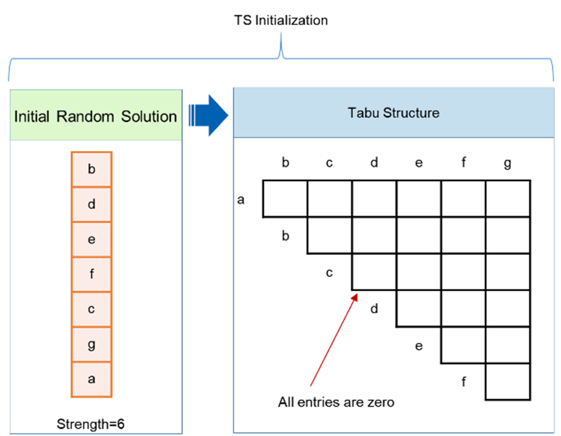
Figure C.20 Composite Laminate Design – Iteration-1
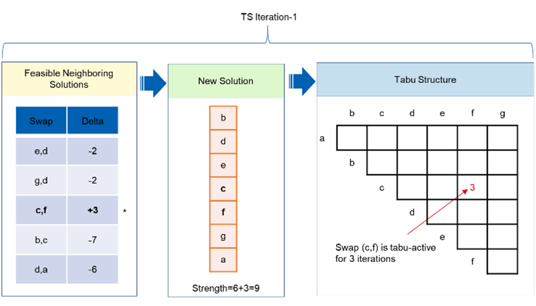
Figure C.21 Composite Laminate Design – Iteration-2
Figure C.22 Composite Laminate Design – Iteration-3
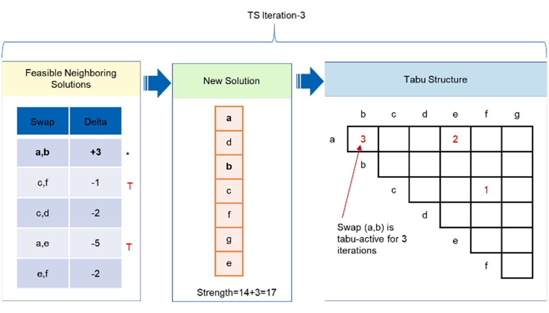
Figure C.23 Composite Laminate Design - TS Iterations 4 and Aspiration Criterion
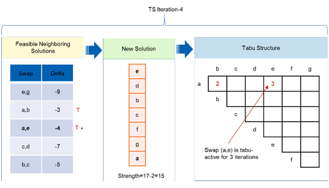
Figure C.24 Frequency-based Memory
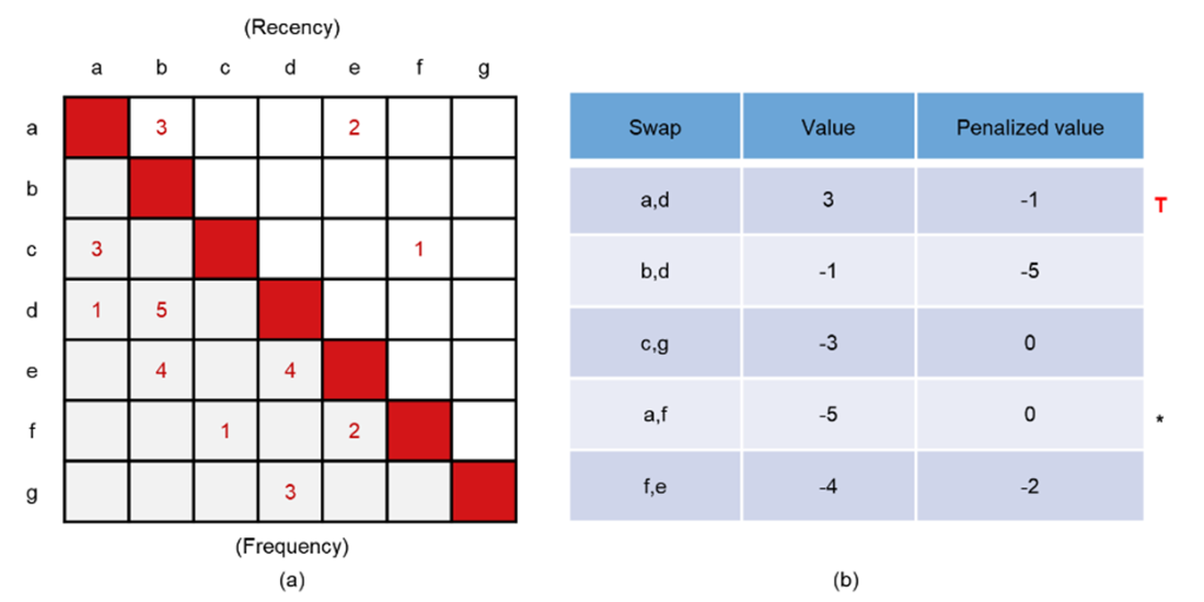
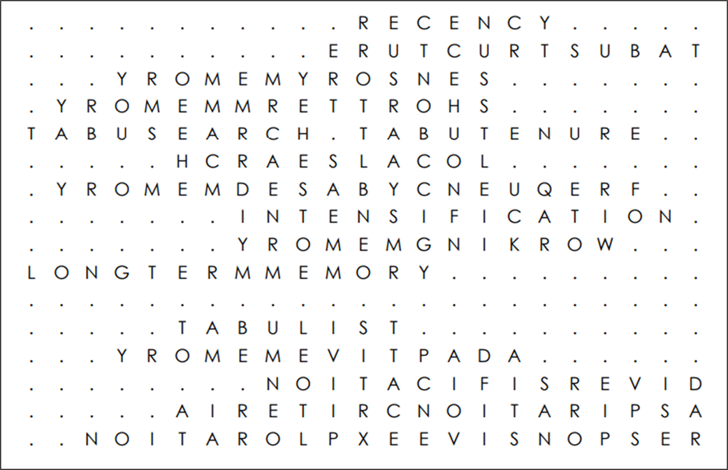
Figure C.25 TS word search puzzle solution
Equation 7.7
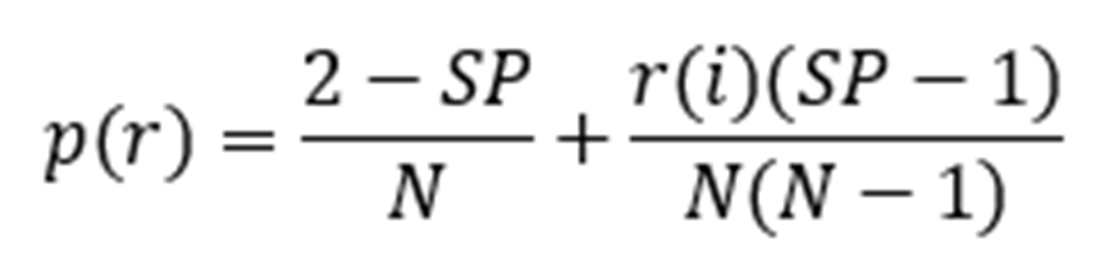
Figure C.26 Ackley function
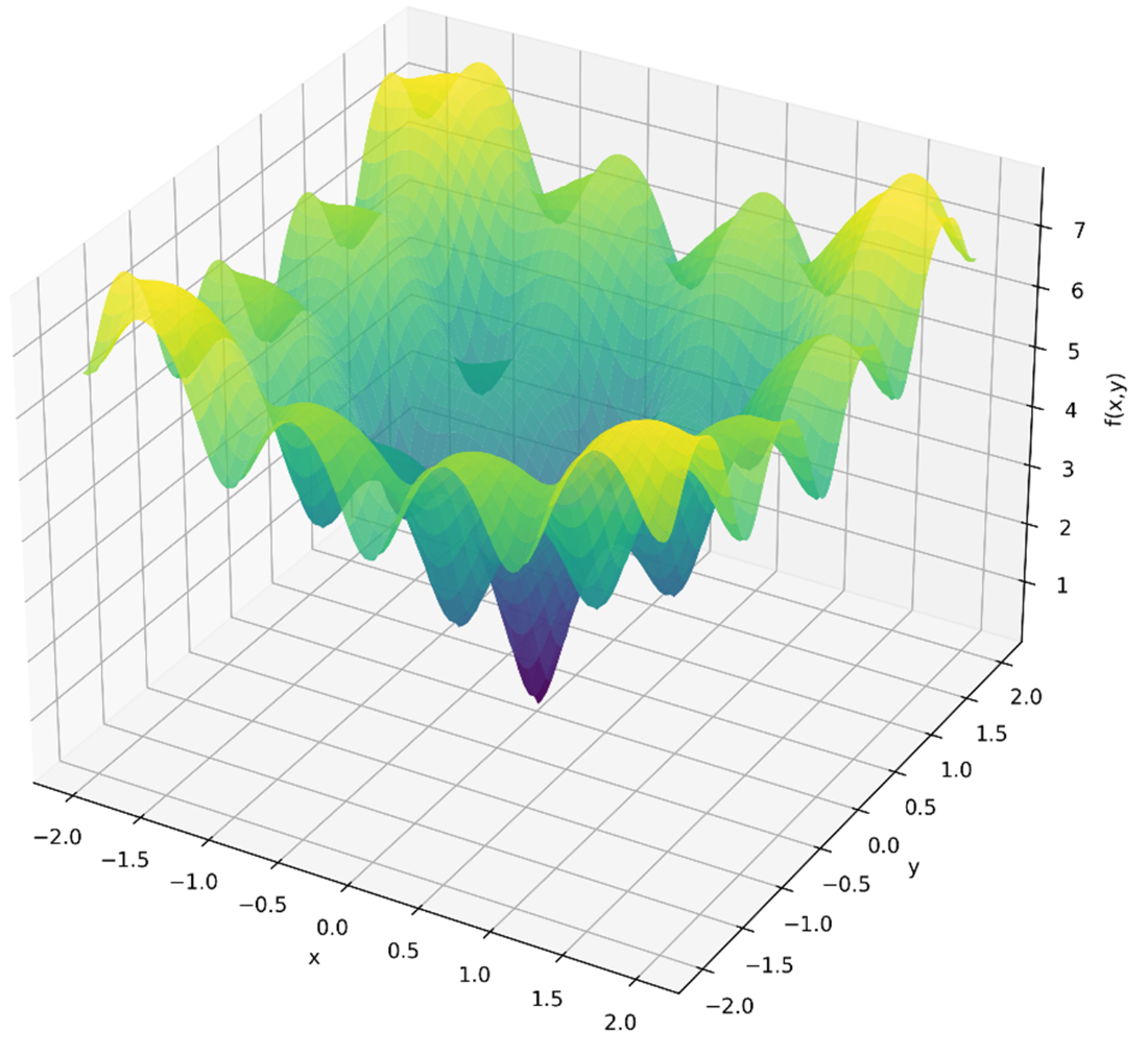
Figure C.27 Cargo bike loading problem for 10 items with given weight, profit and efficiency (profit/weight)
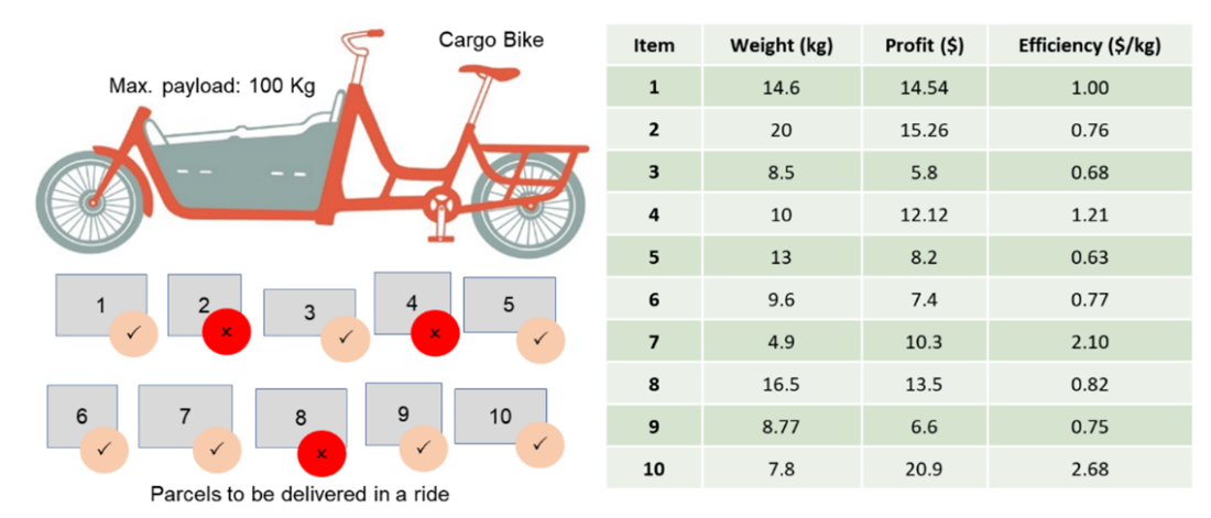
Figure C.28 Opencast mining problem
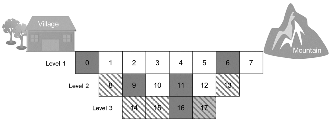
Figure C.29 Cargo bike loading solution
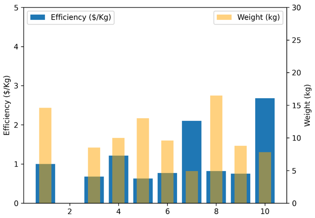
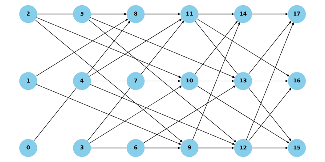
Figure C.30 Precedence graph for extraction of blocks in Level 2 and 3
Equation 9.18
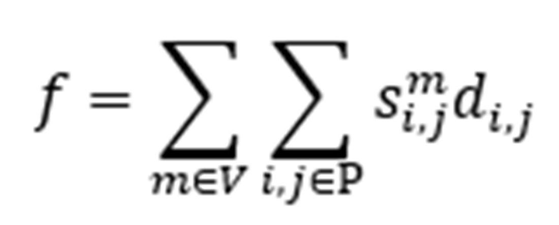
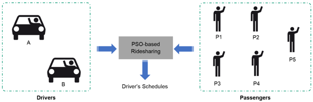
Figure C.31 Ridesharing Problem
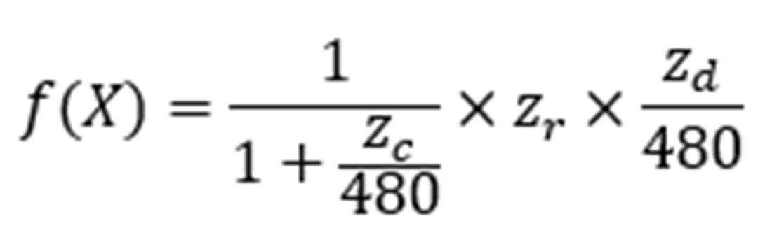
Equation 9.19
Equation 9.20
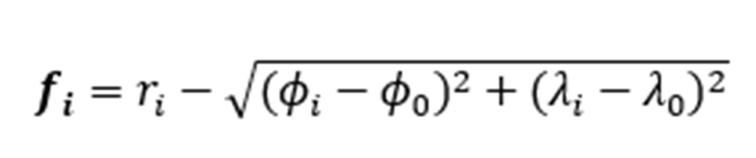
Equation 9.21
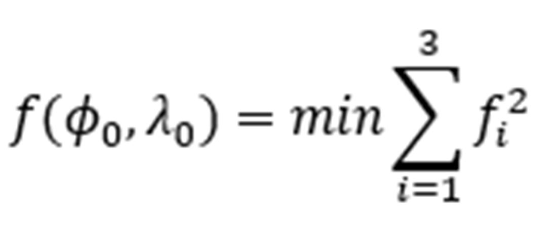
Figure C.32 Cell tower trilateration
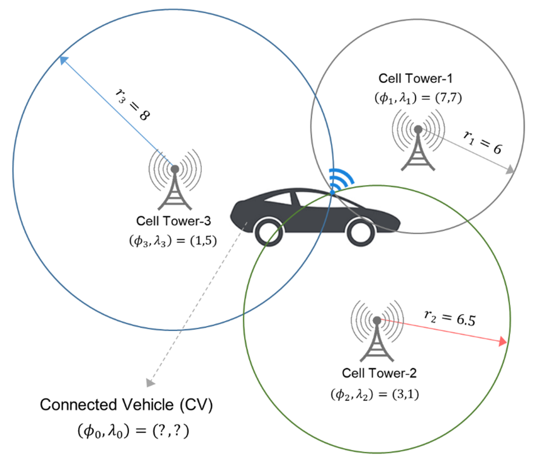
Figure C.33 Hours worked per each doctor
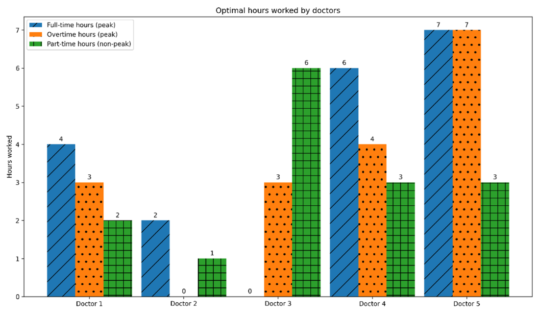
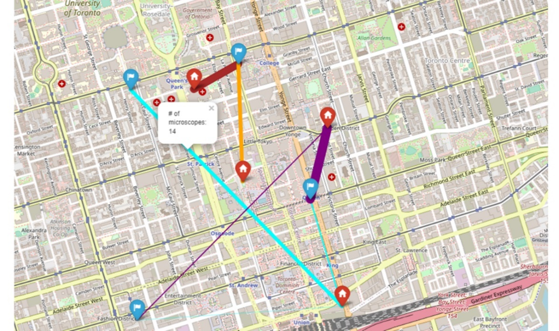
Figure C.34 School microscopes supply-demand
Equation 10.18
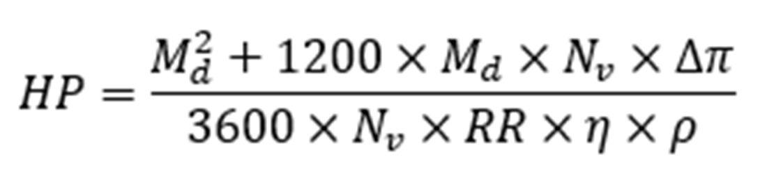
Figure C.35 Optimal route generated by ACO
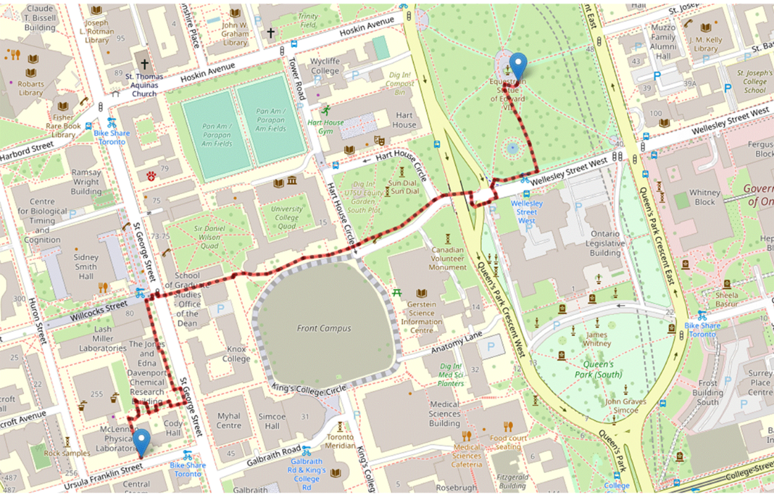
Figure C.36 Supply-demand problem solution obtained by MIDACO
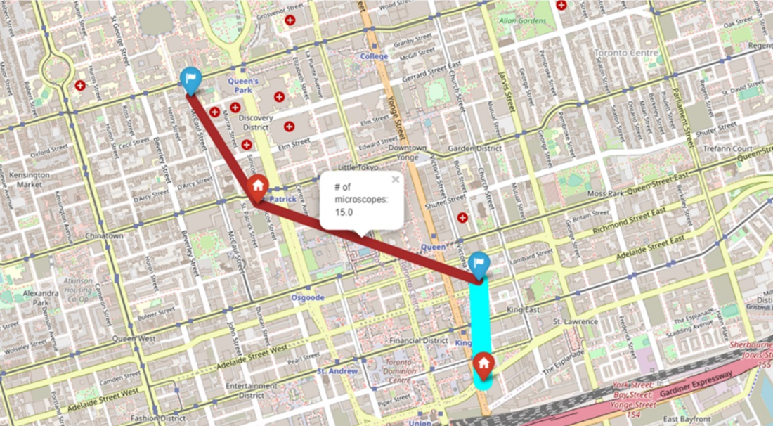
Figure C.37 Progress of SOM training with increasing numbers of iterations.
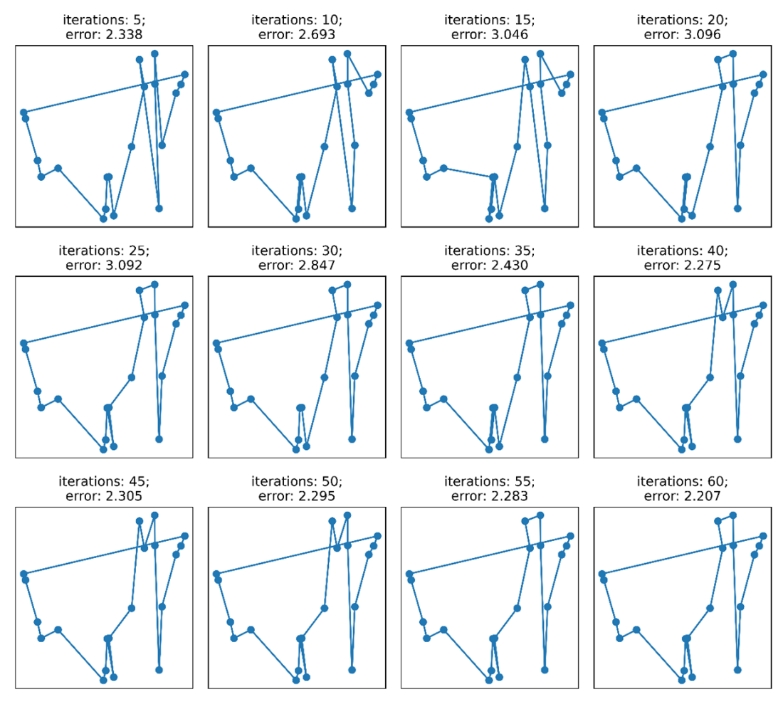
Figure C.38 gym-electric-motor (GEM) Environment [6]
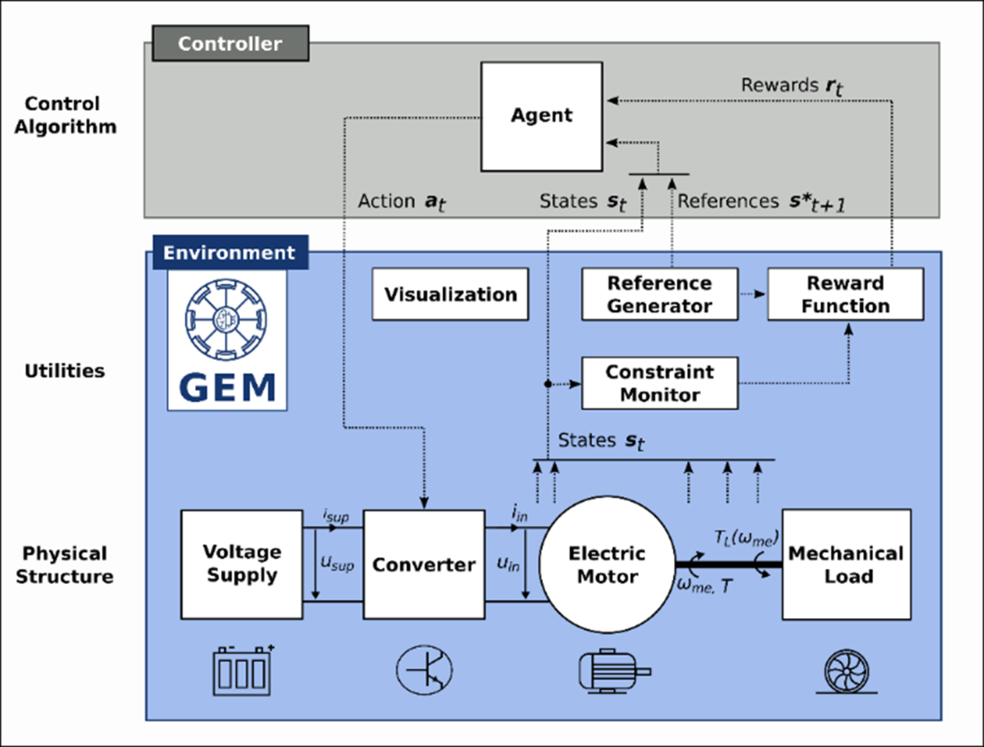
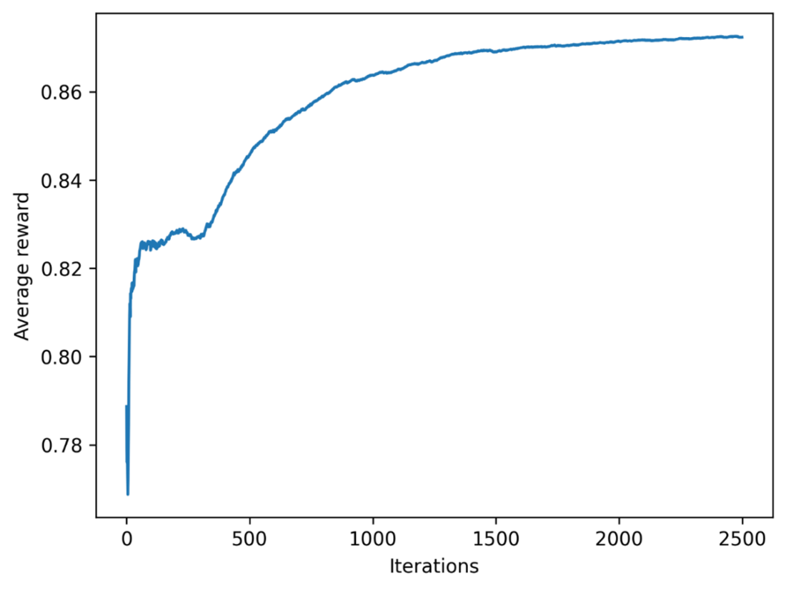
Figure C.39 Average reward in each iteration during the learning process
FAQ

What does Appendix C include and how should I use it?Appendix C gathers exercises and worked solutions for the book’s chapters. You can use it to test understanding (MCQs, T/F), practice modeling and classifying optimization problems, and learn by running provided code snippets (e.g., PuLP, simanneal, pymoo, pyswarms, Stable-Baselines3). Start with the exercises to self-assess, then consult the paired solutions for reasoning, steps, and example implementations.
How do I decide whether a task is a design, planning, or control problem, and whether to use online or offline optimization?- Design: strategic, infrequent, high-quality solution needed (e.g., wind park design, flight scheduling) → offline optimization. - Planning: tactical routing/scheduling under known inputs (e.g., vehicle routing, trip itinerary, school bus loading) → often offline, may be online when frequent re-planning is needed. - Control: real-time adaptation to dynamic changes (e.g., rerouting during motion planning) → online optimization. Many real tasks blend planning (offline) with control (online) for adaptation.
How do I quickly classify an optimization problem (variables, objective, constraints, linearity)?- Decision variables: univariate, bivariate, or multivariate. - Objective: mono-objective or multi-objective (or none → constraint satisfaction). - Constraints: hard (must satisfy), soft (prefer to satisfy), both, or unconstrained. - Linearity: LP (linear), QP (quadratic), NLP (non-linear). Example: “Maximize 3x − y/5 with −2 ≤ x < 3, 0 < y ≤ 3, x + y = 4” → bivariate, mono-objective, hard constraints, linear (LP).
How can I implement the Animal Feed Mix LP in Appendix C (PuLP) and read data from CSV?Steps: - Model: create an LpProblem with objective Minimize total ingredient cost per kg. - Variables: nonnegative decision variables for ingredient proportions. - Constraints: nutritional bounds (e.g., calcium min/max, protein min, fiber max) and conservation (sum of proportions = 1). - Data: define dictionaries in Python or load a CSV to dict and reference columns in constraints/objective. - Solve and report: run the solver, print variable values (percentages) and total cost.
When should I use BFS vs DFS, and when is BFS optimal?- BFS explores by depth levels (FIFO queue), guarantees the shallowest goal, and is optimal when all step costs are equal. - DFS explores deeply first (stack/LIFO), is memory-efficient but risks long detours and missing shallow solutions; it is not optimal in general. - For huge, deep spaces, DFS uses little memory but can expand many nodes; BFS can blow up in memory. Consider Iterative Deepening as a middle ground.
When is A* optimal and what’s the difference between admissible and consistent heuristics?- A* is optimal if h(n) is admissible (never overestimates the true cost-to-go). - Consistency (monotonicity) requires h(n) ≤ cost(n, n′) + h(n′) for all edges; consistent heuristics ensure nondecreasing f-values and simplify implementation. - Greedy best-first uses only h(n), while A* uses f(n) = g(n) + h(n); A* balances path cost and heuristic guidance.
What are the key takeaways about Simulated Annealing and cooling schedules?- Mechanism: allows probabilistic acceptance of worse moves early (high temperature), helping escape local minima; becomes more exploitative as temperature decreases. - Cooling schedules: - Logarithmic: asymptotically convergent but often too slow. - Geometric: practical default (T ← αT), balances speed/quality. - Non-monotonic/adaptive: can reheat or adapt temperature based on progress. - Dual annealing generalizes SA; stochastic hill climbing is a limiting case without thermal jumps.
What should I remember about Tabu Search (TS) memory, aspiration, and tenure tuning?- Memory: - Short-term (recency): tabu list to prevent cycling by forbidding recently used moves. - Long-term (frequency): encourages diversification by penalizing frequent patterns. - Aspiration criteria: override tabu if a move yields a sufficiently good solution. - Tenure: too short → cycling; too long → stagnation. Tune to balance intensification and diversification.
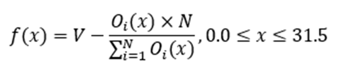
What are practical tips for Genetic Algorithms (GA): encoding, selection, and replacement?- Encoding: binary for parameterized continuous/discrete domains; permutation for order-based problems (e.g., TSP). - Selection: tournament (robust, simple), rank (controls selection pressure), roulette/SUS (fitness-proportionate). - Replacement: generational (replace all) preserves diversity; steady-state (replace few) converges faster. - Bit precision: bits ≈ ceil(log2((range/span)/precision)). Example: 0.0–31.5 at 0.1 precision → 9 bits.
How do I get started with Particle Swarm Optimization (PSO) and what do the velocity terms mean?- Velocity update includes: - Inertia: keeps current motion (exploration). - Cognitive: pull to particle’s best (self-experience). - Social: pull to neighborhood/global best (swarm experience). - Topologies: star/gbest (fast, risk of premature convergence), ring/lbest (slower, more robust). - Using a library (e.g., pyswarms): set objective, bounds, options (w, c1, c2), and run. Choose bounds to reflect variable domains; tune w (explore/exploit tradeoff) and c1/c2 (self vs social pull).

pro $24.99 per month

  • access to all Manning books, MEAPs, liveVideos, liveProjects, and audiobooks!
  • choose one free eBook per month to keep
  • exclusive 50% discount on all purchases
  • renews monthly, pause or cancel renewal anytime

lite $19.99 per month

  • access to all Manning books, including MEAPs!

team

5, 10 or 20 seats+ for your team - learn more


choose your plan

team

monthly
annual
$49.99
$499.99
only $41.67 per month
  • five seats for your team
  • access to all Manning books, MEAPs, liveVideos, liveProjects, and audiobooks!
  • choose another free product every time you renew
  • choose twelve free products per year
  • exclusive 50% discount on all purchases
  • renews monthly, pause or cancel renewal anytime
  • renews annually, pause or cancel renewal anytime
  • Optimization Algorithms ebook for free

choose your plan

team

monthly
annual
$49.99
$499.99
only $41.67 per month
  • five seats for your team
  • access to all Manning books, MEAPs, liveVideos, liveProjects, and audiobooks!
  • choose another free product every time you renew
  • choose twelve free products per year
  • exclusive 50% discount on all purchases
  • renews monthly, pause or cancel renewal anytime
  • renews annually, pause or cancel renewal anytime
  • Optimization Algorithms ebook for free