7 Image Generation with Variational Autoencoders (VAEs)

This chapter introduces variational autoencoders (VAEs) as a practical and conceptually elegant alternative to generative adversarial networks for image generation. It first revisits autoencoders (AEs) to ground the encoder–decoder paradigm, then explains how VAEs extend AEs by learning a probabilistic latent space shaped by a Kullback–Leibler regularizer toward a chosen prior. The result is a continuous, interpretable latent space that enables controllable generation, arithmetic on encodings, and smooth interpolation between inputs. Throughout, the chapter emphasizes the trade-off: AEs and VAEs are simpler and more stable to train than GANs, though their outputs are often less sharp, and highlights practical uses where stability, control, and efficiency matter.

The first project builds an AE to reconstruct handwritten digits. An encoder compresses each image into a low-dimensional latent vector, and a decoder learns to reconstruct the original by minimizing pixel-level reconstruction error. With MNIST data and a compact latent representation, the trained AE produces reconstructions that closely resemble the inputs. However, the chapter underscores key limitations of standard AEs: they tend to map inputs to scattered, non-continuous latent points, which hinders meaningful interpolation and the creation of new, diverse samples beyond those seen in training.

The second project constructs a CNN-based VAE for high-resolution face images. Here, the encoder outputs parameters of a latent distribution (mean and standard deviation), sampling provides latent codes, and training minimizes reconstruction loss plus KL divergence to encourage a well-structured, near-normal latent space. The trained VAE not only reconstructs faces but also generates novel ones by sampling, and it supports intuitive latent operations—such as adding or removing attributes (for example, glasses) through encoding arithmetic and creating smooth transitions via interpolation. The chapter concludes by situating these capabilities in real applications (e.g., product imagery and beyond images to other data types) and by connecting the encoder–decoder design to models explored later in the book.

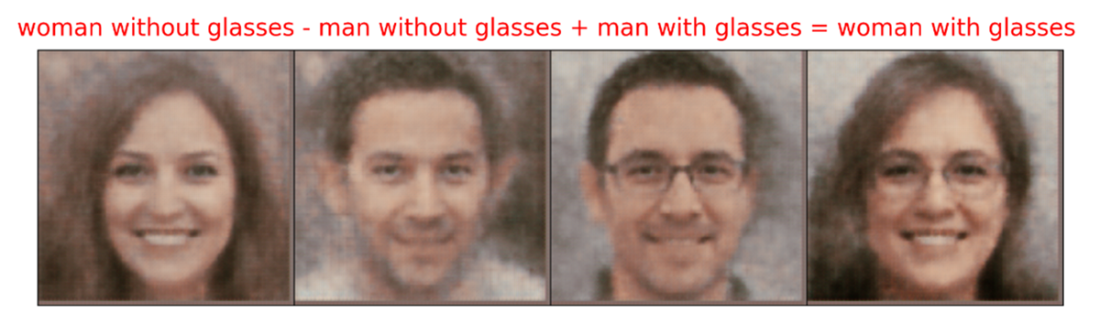
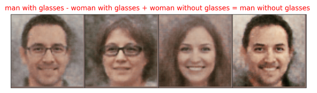
Generating images of women with glasses by performing encoding arithmetic.

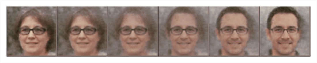
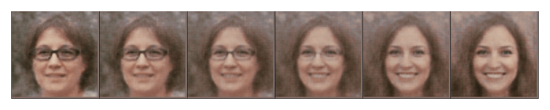
Generating a series of images that transition from glasses with dark frames to those with light frames.

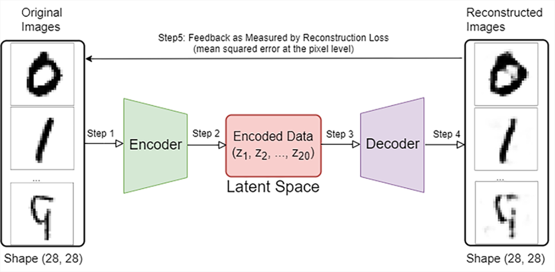
The architecture of an autoencoder (AE) and the steps to train one to generate handwritten digits. An AE consists of an encoder (middle left) and a decoder (middle right). In each iteration of training, images of handwritten digits are fed to the encoder (step 1). The encoder compresses the images to deterministic points in the latent space (step 2). The decoder takes the encoded vectors (step 3) from the latent space and reconstructs the images (step 4). The AE adjusts its parameters to minimize the reconstruction loss: the difference between the originals and the reconstructions (step 5).

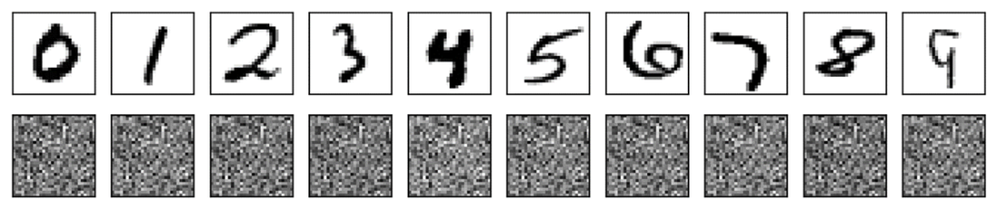
Comparing reconstructed images by the autoencoder with the originals before training starts. The top row shows ten original images of handwritten digits in the test set. The bottom row shows the reconstructed images by the autoencoder before training. The reconstructions are nothing more than pure noise.

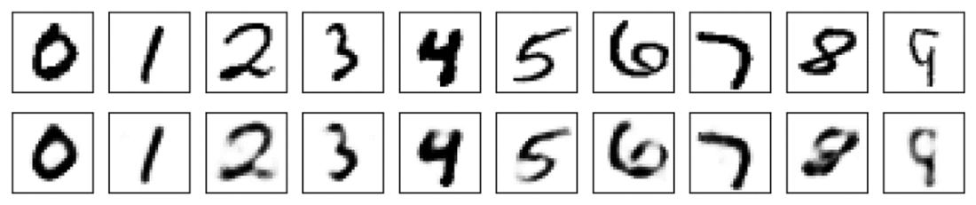
Comparing reconstructed images by the autoencoder with the originals after training. The top row shows ten original images of handwritten digits in the test set. The bottom row shows the reconstructed images by the trained autoencoder. The reconstructed images look similar to the original ones.

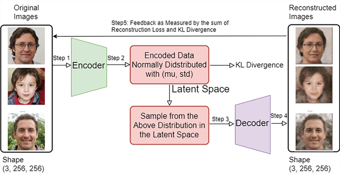
The architecture of a variational autoencoder (VAE) and the steps to train one to generate human face images. A VAE consists of an encoder (middle upper left) and a decoder (middle bottom right). In each iteration of training, human face images are fed to the encoder (step 1). The encoder compresses the images to probabilistic points in the latent space (step 2; since we assume normal distributions, each probability point is characterized by a vector of means and a vector of standard deviations). We then sample encodings from the distribution and present them to the decoder. The decoder takes sampled encodings (step 3) and reconstructs images (step 4). The VAE adjusts its parameters to minimize the sum of reconstruction loss and the Kullback-Leibler (KL) divergence. The KL divergence measures the difference between the encoder’s output and a standard normal distribution.

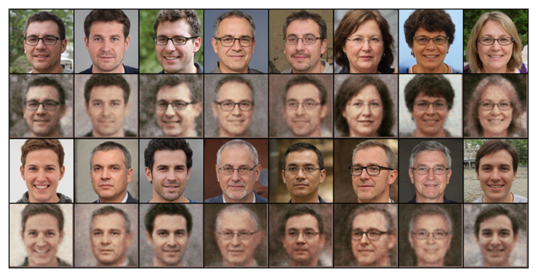
Comparing the reconstructed images by a trained variational autoencoder (VAE) with the originals. The first and the third rows are the original images. We feed them to the trained VAE to obtain the reconstructed images, which are shown below the original images.

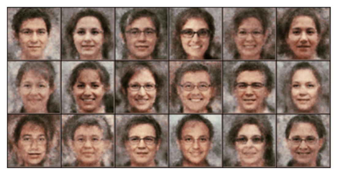
Novel images generated by the trained VAE. We randomly draw vector representations in the latent space and feed them to the decoder in the trained VAE. The decoded images are shown in this figure. Since the vector representations are randomly drawn, the images don’t correspond to any originals in the training set.

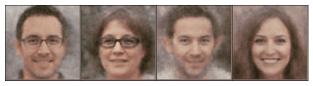
Decoded images based on average encodings. We first obtain three images in each of the following four groups: men with glasses, women with glasses, men without glasses, and women without glasses. We feed the 12 images to the encoder in the trained VAE to obtain their encodings in the latent space. We then calculate the average encoding of the three images in each group. The four average encodings are fed to the decoder in the trained VAE to obtain four images and they are shown in this figure.

An example of encoding arithmetic with the trained VAE. We first obtain the average encodings for the following three groups: men with glasses (z1), women with glasses (z2), and women without glasses (z3). We define a new encoding z=z1-z2+z3. We then feed z to the decoder in the trained VAE and obtain the decoded image, as shown at the far right of this figure.

Interpolating encodings to create a series of intermediate images. We first obtain the average encodings for women with glasses (women_g_encoding) and women without glasses (women_ng_encoding). The interpolated encoding z is defined as w*women_ng_encoding+(1-w)*women_g_encoding, where w is the weight on women_ng_encoding. We change the value of w from 0 to 1 with an increment of 0.2 to create six interpolated encodings. We then decode them and display the resulting six images in the figure.

• Autoencoders (AEs) have a dual-component structure: an encoder and a decoder. The encoder compresses the data into an abstract representation in a lower-dimensional space (the latent space), and the decoder decompresses the encoded information and reconstructs the data.
• Variational autoencoders (VAEs) also consist of an encoder and a decoder. They differ from AEs in two critical ways. Firstly, while an AE encodes each input into a specific point in the latent space, a VAE encodes it into a probability distribution within this space. Secondly, an AE focuses solely on minimizing the reconstruction error, whereas a VAE learns the parameters of the probability distribution for latent variables, minimizing a loss function that includes both reconstruction loss and a regularization term, the Kullback-Liebler (KL) divergence.
• The KL divergence in the loss function when training VAEs ensures the distribution for latent variables resembles a normal distribution. This encourages the encoder to learn continuous, meaningful, and generalizable latent representations.
• A well-trained VAE can map similar inputs to nearby points in the latent space, leading to a more continuous and interpretable latent space. As a result, VAEs can decode random vectors in the latent space into meaningful inputs, leading to outputs that are unseen in the training set.
• The latent space in a VAE is continuous and interpretable, different from that in an AE. As a result, we can manipulate the encodings to achieve new outcomes. We can also create a series of intermediate images transitioning from one instance to another by varying weights on two encodings in the latent space.

FAQ