2 Modeling and measuring latency
This chapter offers a practical framework for thinking about, predicting, and improving latency. It grounds design decisions in two core models: Little’s Law, which links latency, throughput, and concurrency to set realistic performance expectations and guide queue management; and Amdahl’s Law, which quantifies the diminishing returns of parallelism on end-to-end speedups. Crucially, the chapter reframes latency as a distribution rather than a single number, highlighting the importance of tail percentiles for user experience and showing how parallel fanout can amplify the impact of rare slow paths.
The text surveys common sources of latency variability across the stack. Constraints start with physics (distance and speed of light) and continue through CPU and hardware behaviors like caching, branch prediction, speculative execution, SMT contention, and frequency scaling. Virtualization adds hypervisor overhead, resource contention, virtual I/O, and emulation costs; operating systems introduce context switches, interrupts, driver queuing, and firmware pauses. Managed runtimes contribute JIT and GC pauses. Finally, application design choices—algorithms, data access patterns, and concurrency strategies—often dominate what users feel.
It then shows how delays add up and interact: propagation, transmission, processing, and queuing components accumulate; serial stages add directly; parallel and quorum patterns make the slowest contributors (or the minority needed) decisive, elevating tail behavior. For measurement, the chapter emphasizes defining the right perspective (often the user), controlling the environment, and avoiding pitfalls like the observer effect and coordinated omission. It recommends fixed-interval, asynchronous request generation and analyzing distributions with histograms, percentiles, and eCDFs. A simple, timed ping-based exercise illustrates how to capture and visualize a realistic latency distribution without distorting the system under test.
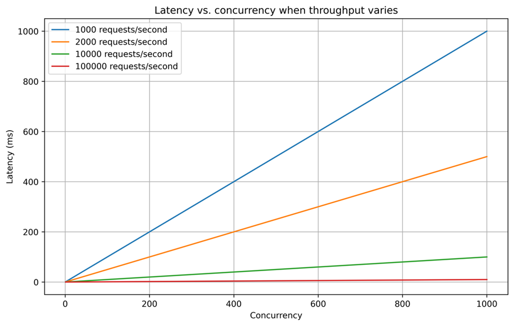
Latency vs concurrency when throughput varies. The diagram shows latency (y-axis) as a function of throughput and concurrency (x-axis).
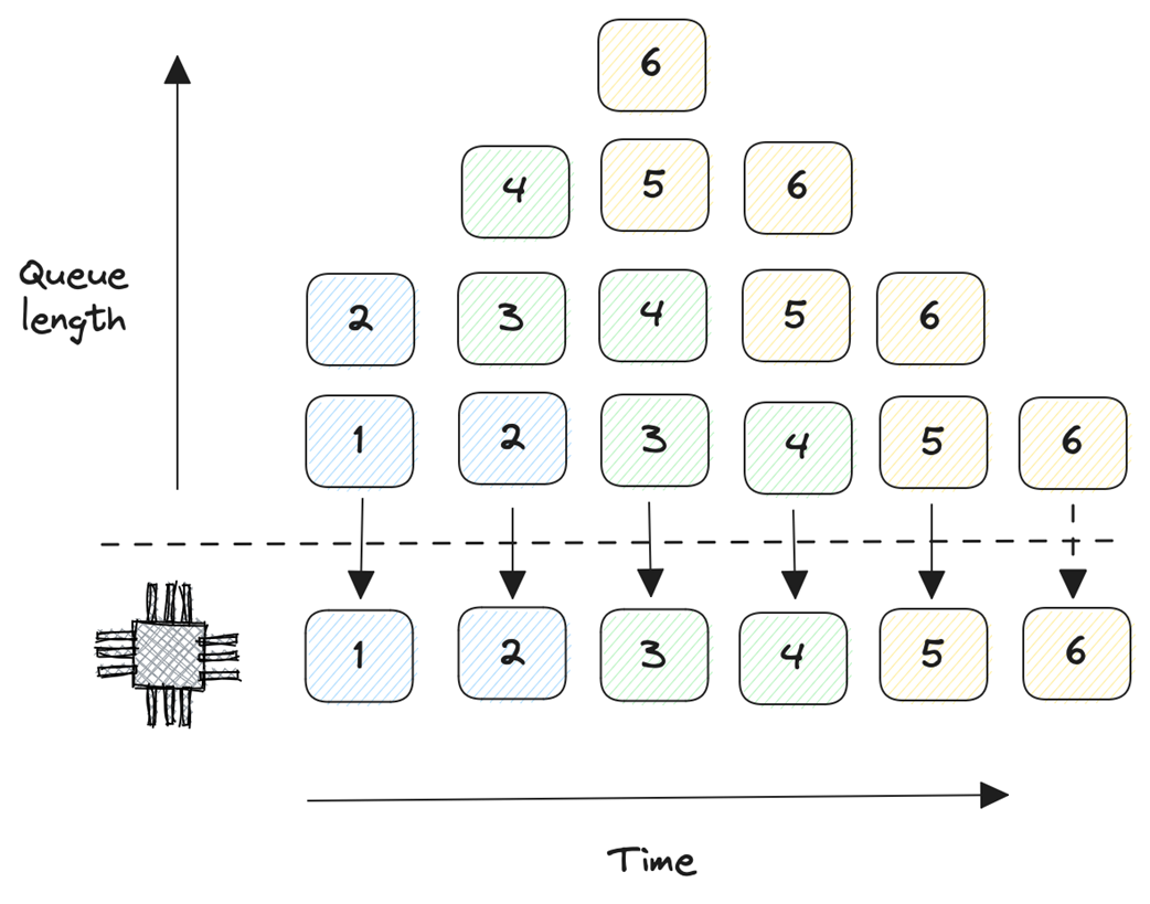
Work arriving to a queue at rate of two tasks per time step with system processing at concurrency of one.
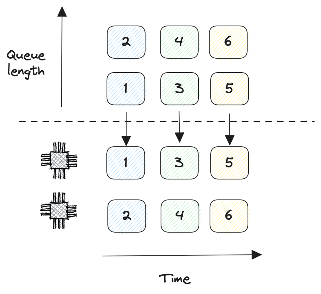
Work arriving to a queue at rate of two tasks per time step with system processing at concurrency of two.
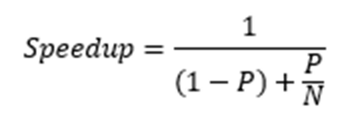
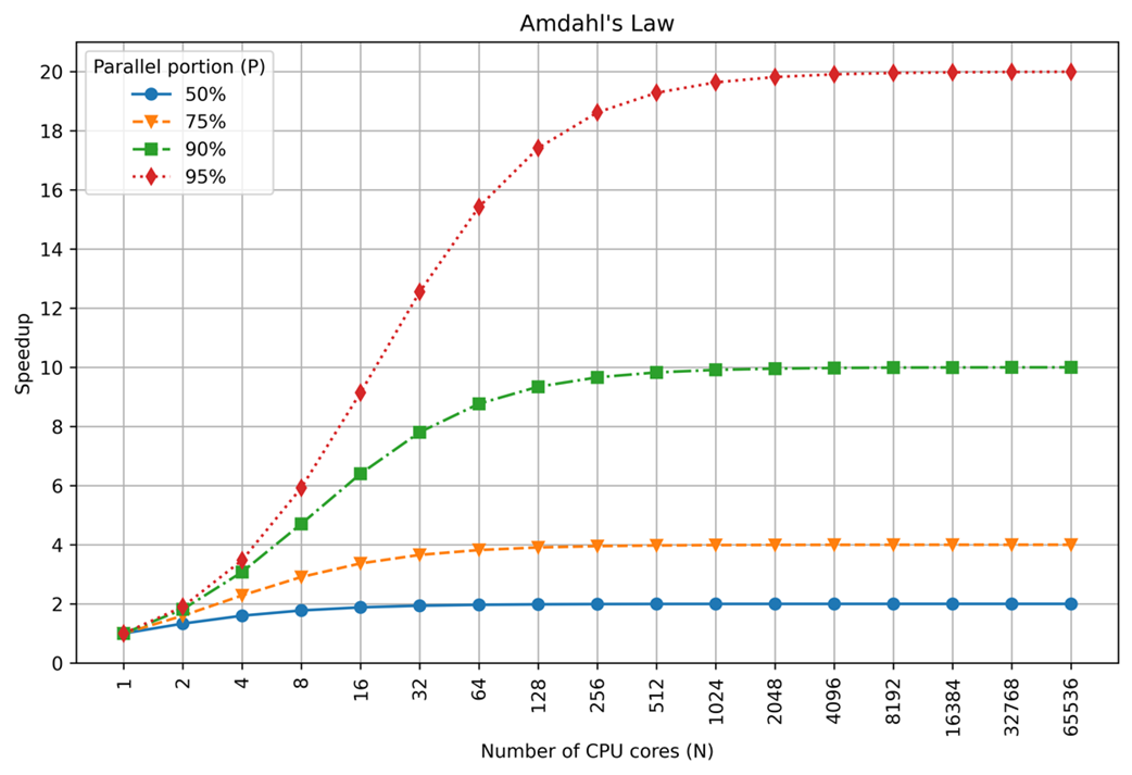
Amdahl’s Law illustrated. The diagram shows theoretical speedup (y-axis) as a function of parallelism (x-axis) given how much of the program is parallelizable.
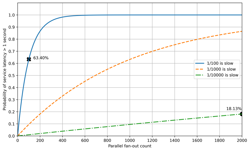
Tail latency illustrated. The diagram shows the probability of service latency being more than 1 second (y-axis) as a function of parallel fanout count (x-axis) depending on the probability of one fanout request being slow.


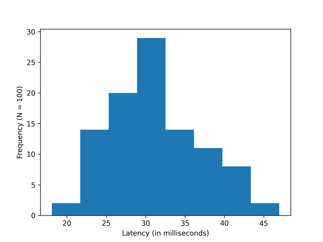
Ping latency histogram.
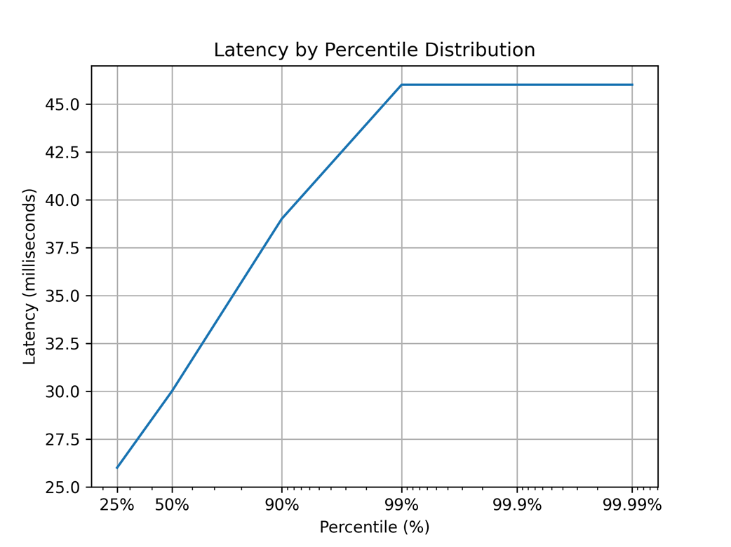
Ping latency HDR histogram.
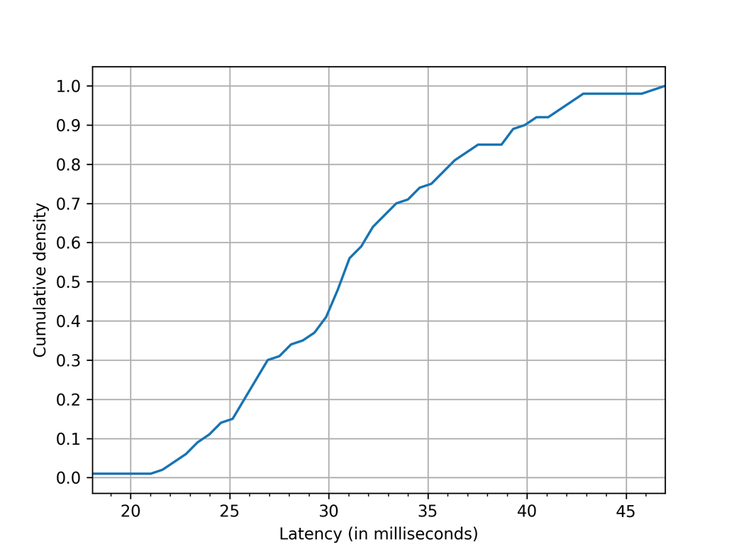
Ping latency eCDF.
Summary
- Little’s Law and Amhdal’s Law are the two fundamental laws of latency, which show the limit how much you can optimize latency. You can use them to reason about how much you can improve the latency in your system, and what is the impact on that on throughput and concurrency.
- Latency is a distribution, not a single value. The high percentile latencies are called the tail latency, which is experienced by users much more often than you think, which is why it’s important to keep tail latency in mind when optimizing your system.
- Tail latency exists because of the variability in latency of your components, which is caused by various factors, from physical limits to operating system configuration and your application design.
- Latency compounds in different ways depending on your design decisions.
- Finally, the key to measuring latency is to define what you are measuring and control your environment accordingly. Histograms and eCDFs are excellent ways to visualize latency.
FAQ
What is Little’s Law and how does it connect latency, throughput, and concurrency?
Little’s Law relates the three via C = T × L, where C is concurrency, T is throughput, and L is average latency. Rearranged, L = C / T. It helps set realistic latency targets given expected throughput and queue sizes. Caution: in real systems, latency often rises with concurrency (due to context switching, locks, etc.), so the law’s simple average-based view can underestimate true concurrency at high load.
How does Amdahl’s Law limit the latency gains from parallelization?
Amdahl’s Law says speedup is bounded by the serial fraction of the work. If a fraction P of a task is parallelizable across N workers, the theoretical speedup levels off as N grows. Even with many cores, serial work dominates. Example: if only 30% is parallelizable, maximum speedup is about 1.4×, so adding cores beyond a point won’t reduce latency meaningfully.
Why is average latency misleading? What should I report instead?
Latency is a distribution, not a single number. Averages hide variability and tail behavior users actually experience. Report percentiles (for example, p50, p90, p95, p99, p99.9) and focus on tail latency. In fan-out systems, overall response time is often determined by the slowest sub-task, so tails matter disproportionately.
What are the main components of end-to-end latency and how do they compound?
- Propagation: distance / signal speed.
- Transmission: packet size / link rate (plus retransmits).
- Processing: active compute time across layers.
- Queuing: time spent waiting in queues (OS scheduler, drivers, services).
Compounding styles:
- Serial compounding: sequential steps add up.
- Parallel compounding: overall latency follows the slowest parallel task.
- Quorum compounding: wait for a majority, not all, which can cut latency versus full fan-in.
What common real-world factors cause latency variability?
- Physics: geographic distance sets lower bounds.
- CPU/hardware: SMT resource contention, cache misses, branch mispredicts, frequency/power scaling.
- Virtualization: hypervisor overhead, noisy neighbors, virtual I/O/switches, hardware emulation.
- OS/drivers/firmware: context switches, interrupts, batching/reordering in drivers, device/CPU firmware activity.
- Managed runtimes: JIT compilation pauses, garbage collection.
- Application design: algorithms, locking, queuing, data access patterns, and dependency chains.
When should I disable SMT (hyperthreading) for low-latency workloads?
Disable SMT when single‑thread tail latency matters and threads contend for shared core resources (execution units, caches, memory bandwidth). Keep it enabled when throughput/efficiency is the priority. Best practice: benchmark with and without SMT, pin critical threads, and choose the setting that meets your tail-latency SLOs.
How should I measure latency to avoid the observer effect?
- Measure from the user’s or caller’s perspective based on your SLO.
- Isolate load generation and metrics collection from the system under test (don’t co‑locate).
- Control environment: client/server placement, background load, and configuration.
- Keep instrumentation lightweight and consistent across runs.
What is coordinated omission and how do I prevent or correct it?
Coordinated omission occurs when a benchmark waits for each response before sending the next. During stalls, fewer requests are issued, so you miss outliers and understate tail latency. Prevent it by sending requests at fixed intervals and handling responses asynchronously. You can also use tools/libraries (for example, HdrHistogram) that correct for expected sampling intervals.
How should I visualize latency distributions?
- Histogram: simple frequency view; can hide tails if binning is coarse.
- Percentile/HDR plots: show key percentiles with high dynamic range for tails.
- eCDF: shows “what fraction completes by X ms” across the full range; great for checking SLO conformance and tail shape.
How can I reduce tail latency in parallel or fan‑out services?
- Reduce fan‑out size; avoid waiting for all subtasks when a quorum suffices.
- Attack variance in components (optimize hot paths, tune GC, improve cache locality, reduce contention).
- Manage queues and backpressure to keep concurrency bounded.
- Use timeouts and budget per sub-task; fail fast or degrade gracefully.

 Latency ebook for free
